På Our World in Data hittar du data med tabeller och över 3000 diagram inom nästan 300 olika områden. Allt är open source och fritt att använda. Ett perfekt ställe att gå till för att faktakolla hur saker och ting ser ut och förhåller sig i världen. Ypperlig källa för att källkritiskt granska påstående om t ex utsläpp, demografisk utveckling, politik, undervisning i olika länder m.m. Det finns även specifika sidor för lärare mer anpassat och paketerat material som kan användas direkt i undervisningen.
Stansning av hål i opaka solceller förvandlar dem till transparenta fönster. Bild från Ulsan National Institute of Science and Technology (UNIST)
Dina kontorfönster kan snart ersättas med solpaneler, eftersom forskare har hittat ett enkelt sätt att göra den gröna tekniken transparent. Tricket är att stansa små hål i dem som är så nära varandra att vi ser dem som tydliga.
Solpaneler kommer att vara avgörande för att öka upptaget av solenergi i städer, säger Kwanyong Seo vid Ulsan National Institute of Science and Technology, Sydkorea.
Det beror på att takutrymmet förblir relativt fast medan fönsterutrymmet växer när byggnader blir högre. ”Om vi applicerar transparenta solceller på fönster i byggnader kan de generera enorma mängder elkraft varje dag,” säger Seo.
Problemet med de senaste utvecklade transparenta solcellerna är att de ofta är mindre effektiva. De tenderar också att ge ljuset som passerar genom dem en röd eller blå nyans.
För att övervinna detta söker många forskare efter nya material att bygga transparenta solceller med. Seo och hans kollegor ville dock utveckla transparenta solceller från det mest använda materialet, kristallina kiselskivor, som finns i cirka 90 procent av solcellerna över hela världen.
De tog 1 centimeter kvadratceller gjorda av kristallint kisel, som är helt ogenomskinligt, och sedan stansade små hål i dem för att släppa igenom ljuset.
Hålen är 100 mikrometer i diameter, omkring storleken på ett mänskligt hår, och de släpper igenom 100 procent av ljuset utan att ändra färg.
Den fasta delen av cellen absorberar fortfarande allt ljus som träffar den, vilket resulterar i en hög effektomvandlingseffektivitet på 12 procent. Detta är väsentligt bättre än de 3 till 4 procent som andra transparenta celler har uppnått, men är fortfarande lägre än 20 procent effektiviteten som de bästa helt ogenomskinliga cellerna som för närvarande finns på marknaden.
Under de kommande åren hoppas Seo och hans kollegor att utveckla en solcell som har en effektivitet på minst 15 procent. För att kunna sälja dem på marknaden måste de också utveckla en elektrod som är transparent.
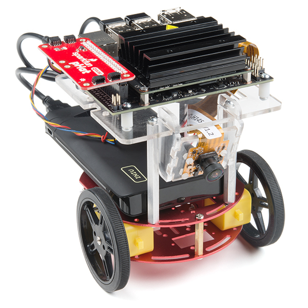
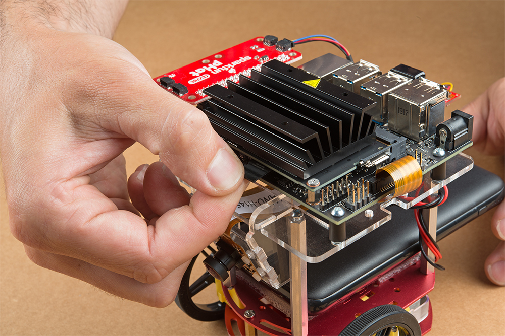
SparkFun’s version of the JetBot merges the industry leading machine learning capabilities of the NVIDIA Jetson Nano with the vast SparkFun ecosystem of sensors and accessories. Packaged as a ready to assemble robotics platform, the SparkFun JetBot Kit requires no additional components or 3D printing to get started – just assemble the robot, boot up the Jetson Nano, connect to WiFi and start using the JetBot immediately. This combination of advanced technologies in a ready-to-assemble package makes the SparkFun JetBot Kit a standout, delivering one of the strongest robotics platforms on the market. This guide serves as hardware assembly instructions for the two kits that SparkFun sells; Jetbot including Jetson Nano & the Jetbot add-on kit without the NVIDIA Jetson Nano. The SparkFun JetBot comes with a pre-flashed micro SD card image that includes the Nvidia JetBot base image with additional installations of the SparkFun Qwiic Python library, Edimax WiFi driver, Amazon Greengrass, and the JetBot ROS. Users only need to plug in the SD card and set up the WiFi connection to get started.
Note: We recommend that you read all of the directions first, before building your Jetbot. However, we empathize if you are just here for the pictures & a general feel for the SparkFun Jetbot. We are also those people who on occasion void warranties & recycle unopened instructions manuals. However, SparkFun can only provide support for the instructions laid out in the following pages.
Attention: The SD card in this kit comes pre-flashed to work with our hardware and has the all the modules installed (including the sample machine learning models needed for the collision avoidance and object following examples). The only software procedures needed to get your Jetbot running are steps 2-4 from the Nvidia instructions (i.e. setup the WiFi connection and then connect to the Jetbot using a browser). Please DO NOT format or flash a new image on the SD card; otherwise, you will need to flash our image back onto the card.
If you accidentally make this mistake, don’t worry. You can find instructions for re-flashing our image back onto the SD card in the software section of the guide
The Jetson Nano Developer Kit offers extensibility through an industry standard GPIO header and associated programming capabilities like the Jetson GPIO Python library. Building off this capability, the SparkFun kit includes the SparkFun Qwiic pHat for Raspberry Pi, enabling immediate access to the extensive SparkFun Qwiic ecosystem from within the Jetson Nano environment, which makes it easy to integrate more than 30 sensors (no soldering and daisy-chainable).
The SparkFun Qwiic Connect System is an ecosystem of I2C sensors, actuators, shields and cables that make prototyping faster and less prone to error. All Qwiic-enabled boards use a common 1mm pitch, 4-pin JST connector. This reduces the amount of required PCB space, and polarized connections mean you can’t hook it up wrong.
Materials
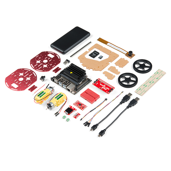
The SparkFun Jetbot Kit contains the following pieces; roughly top to bottom, left to right.
Part
Qty
Circular Robotics Chassis Kit (Two-Layer)
1
Lithium Ion Battery Pack – 10Ah (3A/1A USB Ports)
1
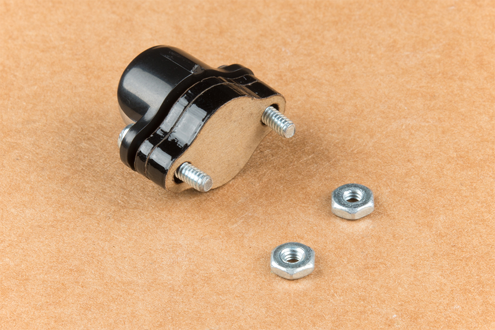
Ball Caster Metal – 3/8″
1
Edimax 2-in-1 WiFi and Bluetooth 4.0 Adapter
1
Header – male – PTH – 40 pin – straight
1
2 in – 22 gauge solid core hookup wire (red)
1
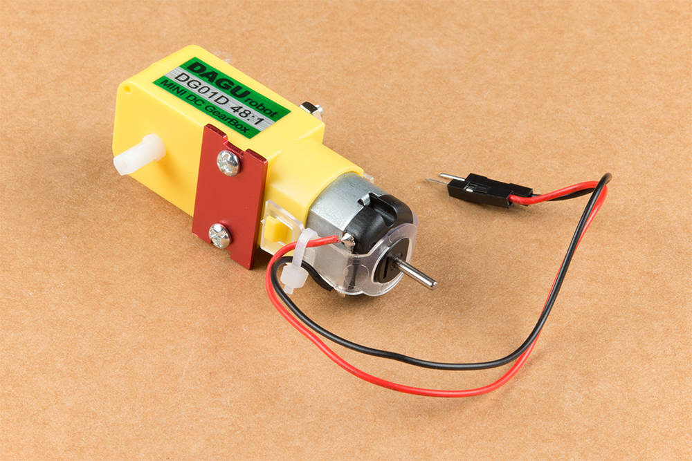
Shadow Chassis Motor (pair)
1
Jetson Dev Kit (Optional)
1
SparkFun JetBot Acrylic Mounting Plate
1
SparkFun Jetbot image (Pre Flashed)
1
Leopard Imaging 145 FOV Camera
1
Screw Terminals 2.54mm Pitch (2-Pin)
2
SparkFun Micro OLED Breakout (Qwiic)
1
SparkFun microB USB Breakout
1
SparkFun Serial Controlled Motor Driver
1
Breadboard Mini Self-Adhesive Red
1
SparkFun Qwiic HAT for Raspberry Pi
1
SparkFun JetBot Acrylic sidewall for camera mount
2
SparkFun JetBot Acrylic Camera mount & 4x nylon mounting hardware
1
Qwiic Cable – 100mm
1
Qwiic Cable – Female Jumper (4-pin)
1
Wheels & Tires – included as part of circular robotics chassis
2
USB Micro-B Cable – 6″
2
Dual Lock Velcro
1
The SparkFun Jetbot Kit contains the following hardware; roughly top to bottom, left to right.
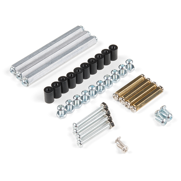
We did not include any tools in this kit because if you are like us you are looking for an excuse to use the tools you have more than needing new tools to work on your projects. That said, the following tools will be required to assemble your SparkFun Jetbot.
Small phillips & small flat head head screwdriver will be needed for chassis assembly & to tighten the screw terminal connections for each motor. We reccomend the Pocket Screwdriver Set; TOL-12268.
Pair of scissors will be needed to cut the adhesive Dual Lock Velcro strap to desired size; recommended, but not essential..
Soldering kit for assembly & configuration of the SparkFun Serial Controlled Motor Driver – example TOL-14681
Optional– adjustable wrench or pliers to hold small components (nuts & standoffs) in place while tightening screws; your finger grip is usually enough to hold these in place while tightening screws & helps to ensure nothing is over tightened.A Note About Directions
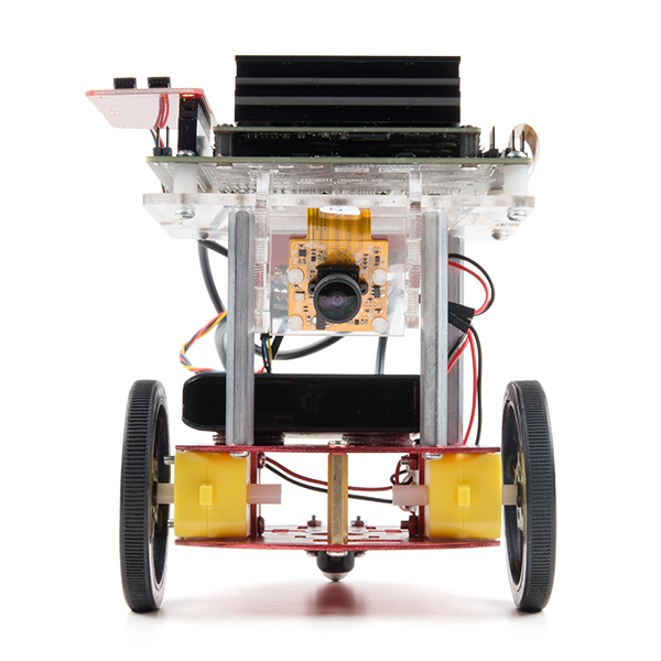
When we talk about the ”front,” or ”forward” of the JetBot, we are referring to direction the camera is pointed when the Jetbot is fully assembled. ”Left” and ”Right” will be from the perspective of the SparkFun Jetbot.
If you prefer to follow along with a video, check out this feature from the chassis product page. You do not need to use the included ball caster as a larger option has been provided for smoother operation.
Start by attaching the chassis motor mount tabs to each of the ”Shadow Chassis Motors (pair)” using the long threaded machine screws & nuts included with the Circular Robotics Chassis Kit.
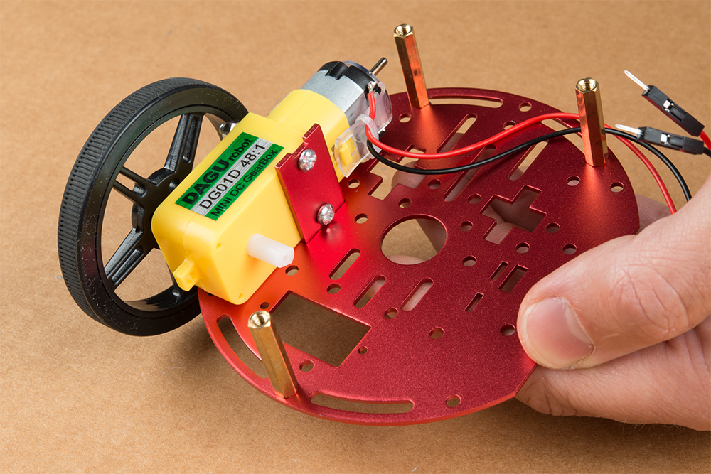
Fit the rubber wheels onto the hubs, install the wheel onto each motor, & fix them into position using the self tapping screws included with the Circular Robotics Chassis Kit.
Install the brass colored standoffs included with the Circular Robotics Chassis Kit; two in the rear and one in the front. The rear of the SparkFun Jetbot will be on the side of the plate with the two ”+” sign cut outs. The rear of the motor will be opposite the wheel where the spindle extends. This orientation ensures the widest base & most stable set up for your Jetbot.
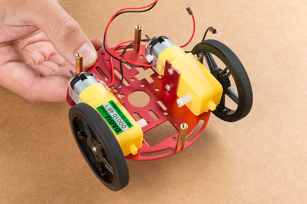
The motor mounts fit into two mirrored inlets in each base plate as shown. Install the motors opposite of one another.
Depending on how you install the motor mounts to each motor will dictate how the motor can be installed on the base plate. Note: Do not worry about the motor orientation as you will determine proper motor operation in how you connect the motor leads to the SparkFun Serial Controlled Motor Driver. Notice how in the picture below one motor has the label facing up, while the other has the label facing down.
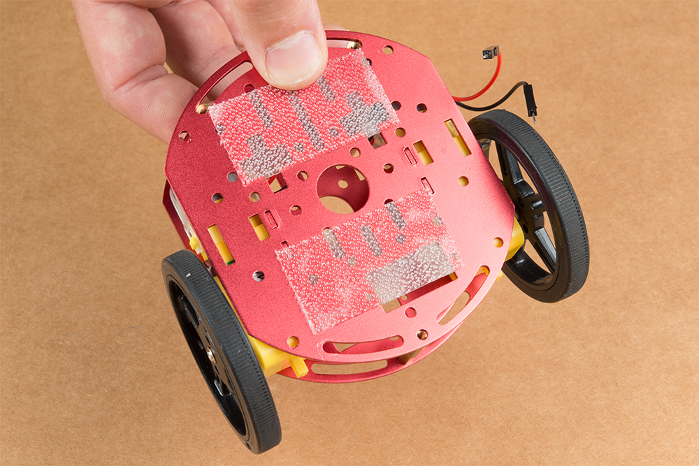
Place the other circular robot chassis plate on top of and align the two ”+” and the motor mount tab recesses. Hold the sandwiched chassis together with one hand and install the remaining Phillips head screws included with the Circular Robotics Chassis Kit through the top plate & into the threaded standoffs.
Your main chassis is now assembled! The Circular Robotics Chassis Kit also contains a very small caster wheel assembly, but we have included a larger metal caster ball to increase the stability of the SparkFun Jetbot. We will cover the installation of this caster ball later in the tutorial.
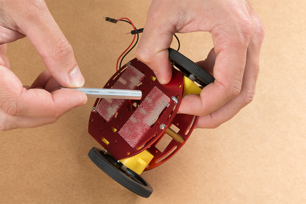
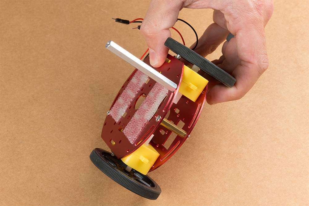
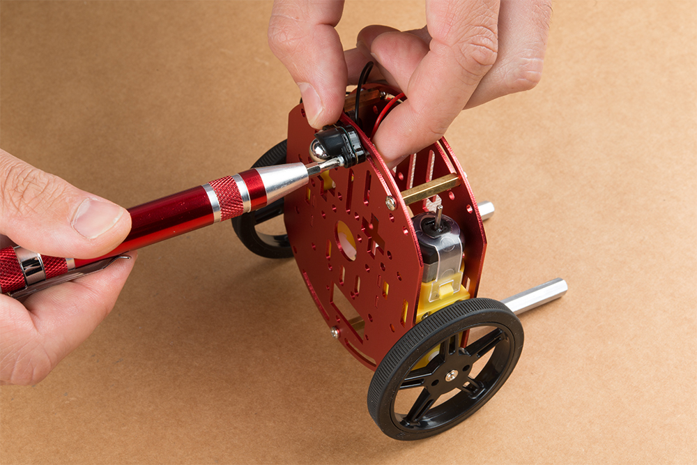
Utilize three of the included 1/4 in 4-40 Phillips Screws through the top chassis plate with threads facing up & install the 2-3/8 in #4-40 Aluminum Hex Standoff until they are finger tight.
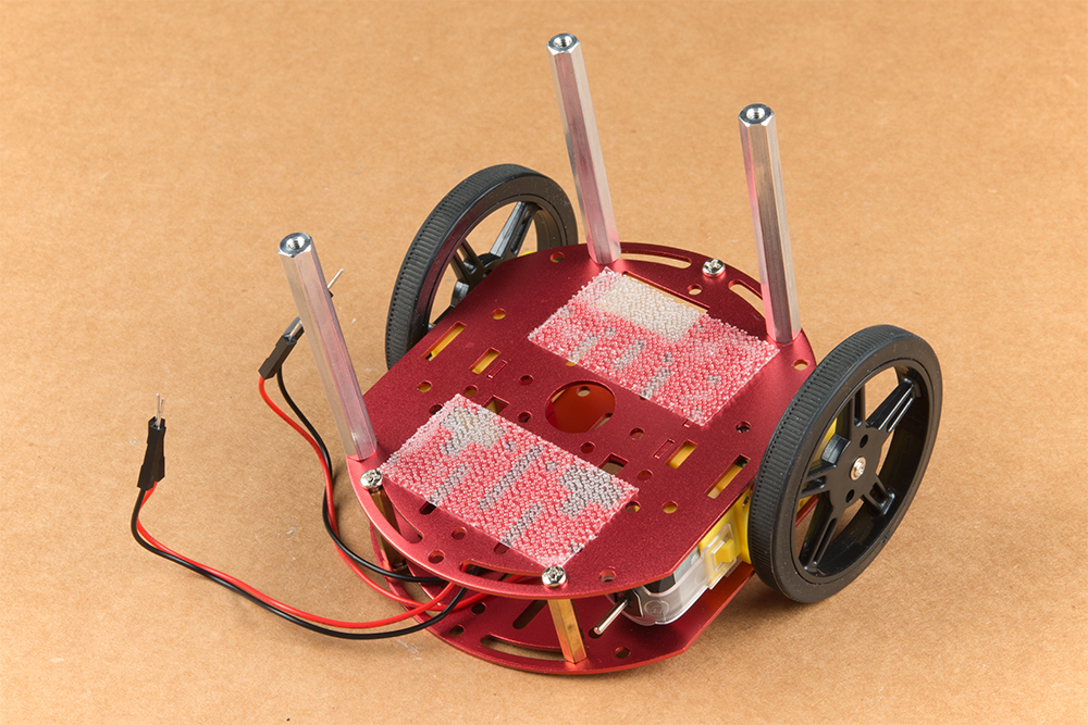
The aluminum stand offs should be pointing up as shown below.
The SparkFun JetBot acrylic mounting plate is designed to have two of these aluminum standoffs in the front & one in the rear. We recommend the rear standoff on the left side of the chassis (as shown) so the 6 in microB usb cables that will be installed later can more easily span the gap needed to power the JetBot.
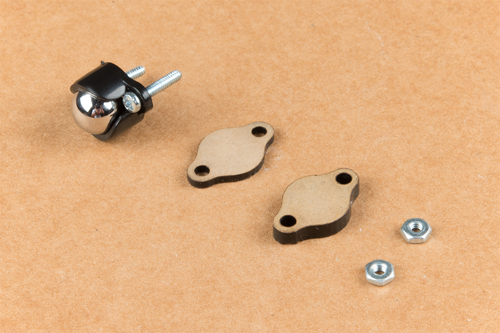
Un-package the 3/8 in Metal Caster Ball and thread the mounting screws through all pieces as shown. Note the full stack height will help balance the Jetbot in a stable position.
Install the caster wheel using the Phillips head screws and nuts included with the 3/8 in caster ball assembly. The holes on the caster assembly are spaced to fit snug on the innermost segment of the angular slots near the rear of the lower plate on the JetBot chassis. Again, hand tight is just fine. Note: if you over tighten these screws it will prevent the ball from easily rotating in the plastic assembly. However, too loose and it may un-thread; go for what feels right
After you have installed the caster & aluminum standoffs, thread the motor wires through the back of the chassis standoffs for use later.
2. Camera Assembly & Installation
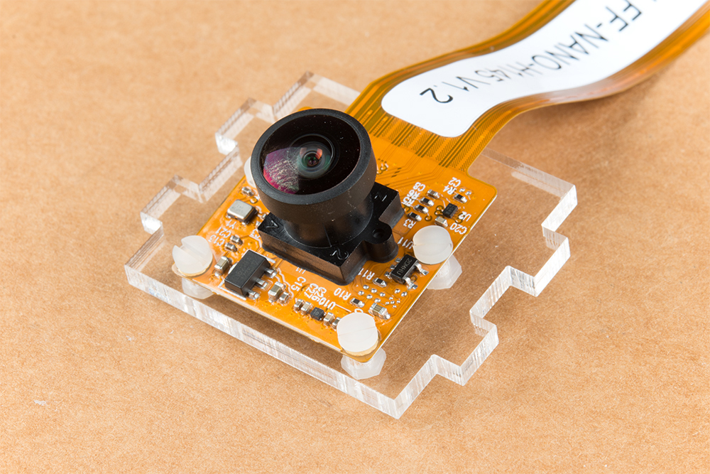
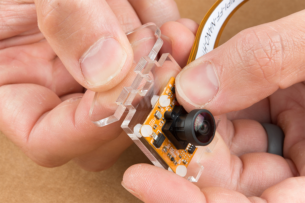
Unpackage the Leopard Imaging camera & align the four holes in the acrylic mounting plate with those on the camera.
Note: ensure that the ribbon cable is extending over the acrylic plate on the edge that does not have mounting holes near the edge; as shown below.
Place all four nylon flathead screws through the camera & acrylic mounting plate prior to fully tightening the nylon nuts. This will ensure equal alignment across all four screws. Tighten the screws while holding the nuts with finger pressure in a rotating criss cross pattern; similar to how you tighten lug nuts on a car rim.
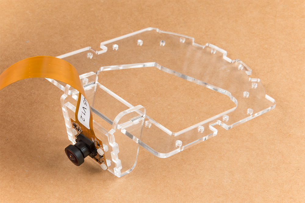
Align one acrylic sidewall with the camera mounting plate as shown below ensuring that the widest section of the sidewall is oriented to the top of the camera mount where the ribbon cable extends.
Apply even pressure on each piece until they fit together. Note: these pieces are designed to have an interference fit and will have a nice, satisfying ”click” when they fit together.
Repeat this process on the other side to fully assemble the camera mount.
The camera mount should now be installed to the SparkFun Jetbot acrylic mounting plate using the overlapping groove joints. Ensure that the cut out on the acrylic mounting plate is facing towards the front/right of the Jetbot as shown. This will ensure that there is plenty of room for the camera ribbon cable to pass around the assembly and up to the Jetson nano camera connector.
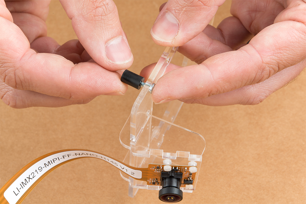
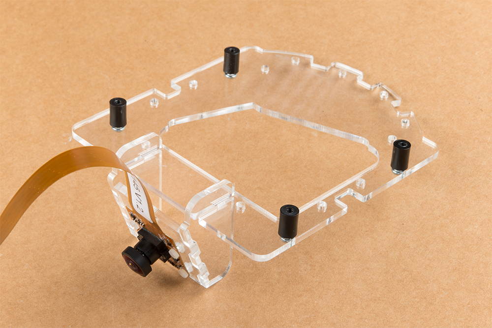
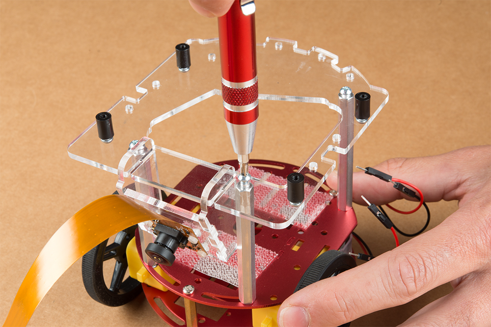
Install four of the nylon standoffs to the top of the SparkFun Jetbot acrylic mounting plate using four of the included 1/4 in 4-40 Phillips head screws as shown below.
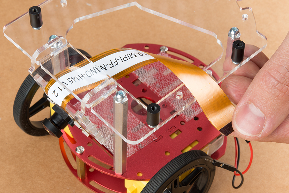
Utilize three more of the 1/4 in 4-40 Phillips head screws to install the SparkFun Jetbot acrylic mounting plate to the aluminum standoffs extending from the Two-layer circular robotics chassis as shown below.
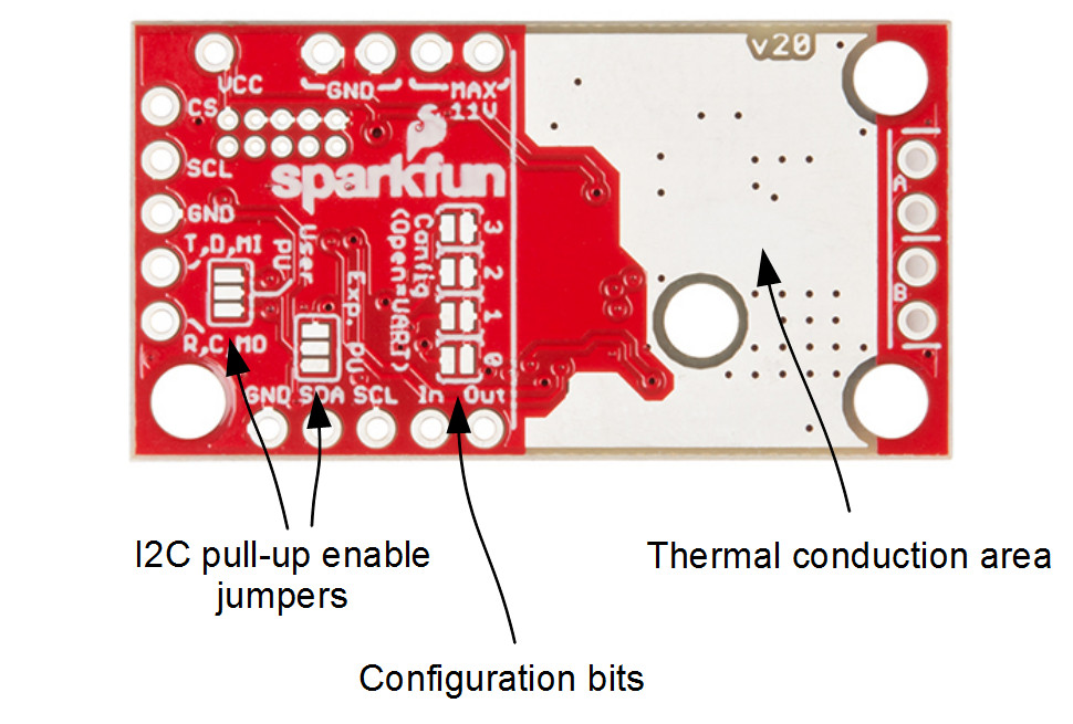
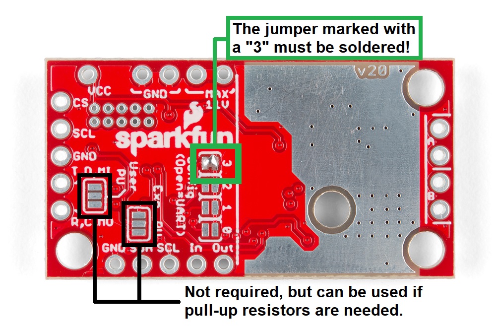
You will need to solder both triple jumpers labeled below as ”I2C pull-up enable jumpers” as the SparkFun pHat utilizes the I2C protocol. The default I2C address that is used by the pre-flashed SparkFun Jetbot image is 0x5D which is equavalent to soldering pad #3 noted as ”configuration bits” on the back of the SparkFun serial controlled motor driver; see below. You will need to create a solder jumper on pad #3 only for the SparkFun Jetbot Image to work properly.
Layout of jumpers on the Serial Controlled Motor Driver.
Jumper 3 of theConfiguration Bitsproperly soldered.
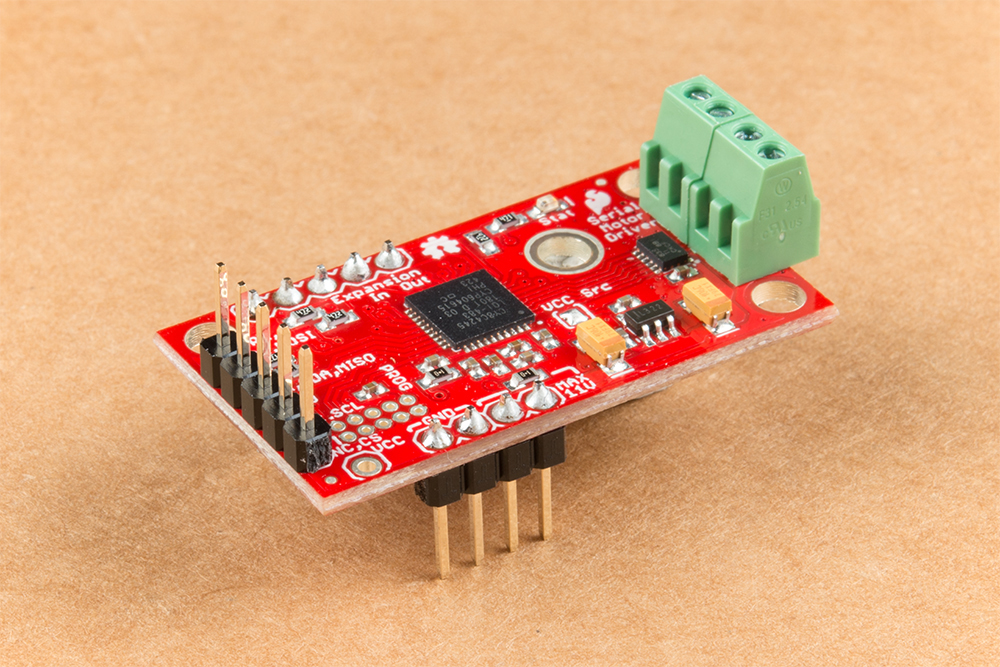
Your completed Serial Controlled motor drive should look somewhat similar to the board shown below.
The 2-pin screw terminals are soldered to the ”Motor Connections.”
Break off 4 Male PTH straight headers and solder into the ”Power (VIN) connection” points.
Break off 5 Male PTH straight headers and solder into the ”Expansion port” points. These will not be used, but will provide additional board stability when installed into the mini breadboard.
Break off 5 Male PTH straight headers and solder into the ”User port” points for connection into the included Female Jumper Qwiic cables.
Break off 5 Male PTH straight headers and solder into the breakout points on the SparkFun microB USB Breakout.
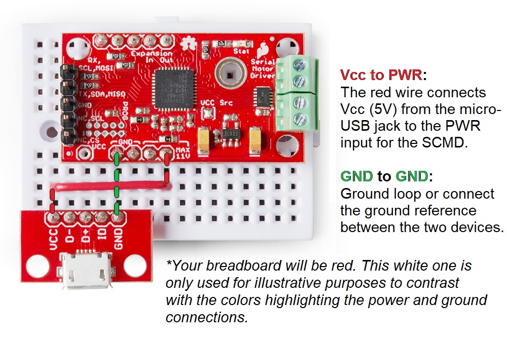
Install both the SparkFun Serial Controlled Motor Driver & the SparkFun microB Breakout board on the included mini breadboard so the ”GRD” terminals for each unit share a bridge on one side of the breadboard.
Utilize the included 2 in – 22 gauge solid core hookup wire (red) to bridge the ”VCC” pin for the SparkFun microB Breakout to either (VIN) connection point on the SparkFun Serial Controlled Motor Driver as shown below.
Required power connections between the micro-USB breakout and the Serial Controlled Motor Driver.
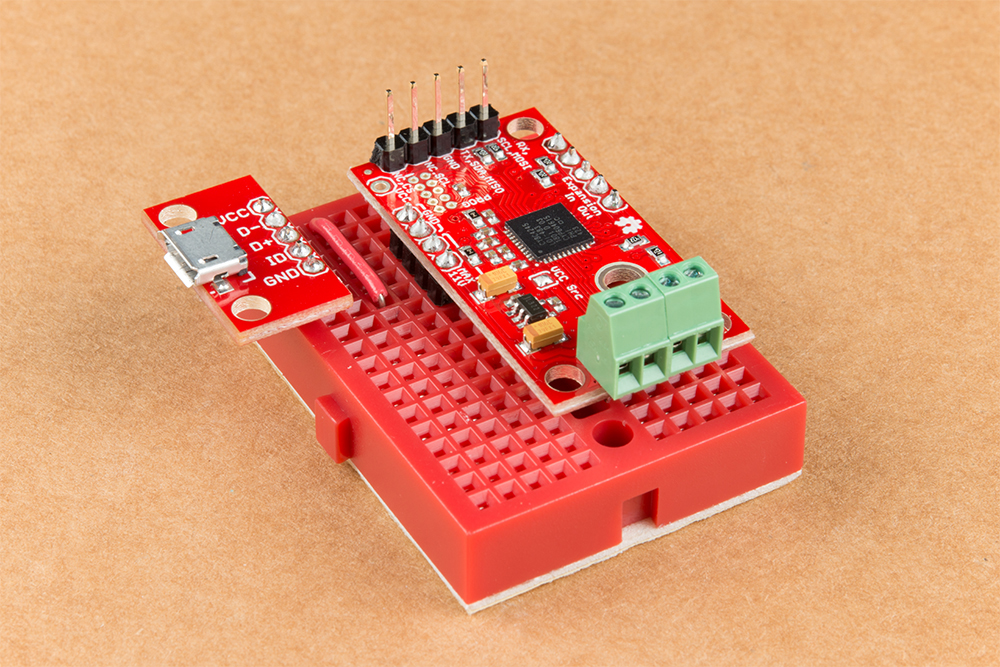
Competed assembly of the micro-USB breakout and Serial Controlled Motor Driver on the breadboard.
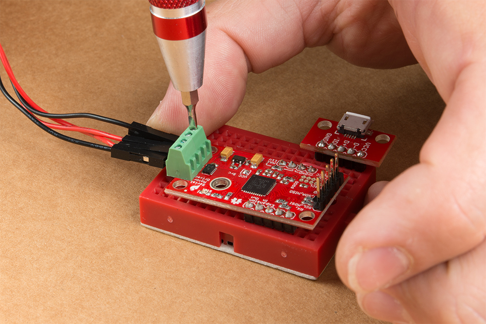
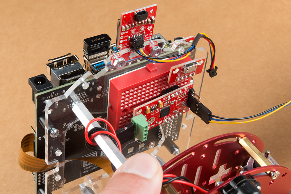
Utilize a small flat head screwdriver to loosen the four connection points on the screw terminals. When inserting the motor connection wires, note the desired output given the caution noted in section #1 of this assembly guide.
Note from section #1: Do not worry about the motor orientation as you will determine proper motor operation in how you connect the motor leads to the SparkFun Serial Controlled Motor Driver.
These connection points can be corrected when testing the robot functionality. If your Jetbot goes straight when you expect Jetbot to turn or vice versa, your leads need to be corrected.
Set this assembly aside for full installation later.
4. Accessory Installation to Main Chassis
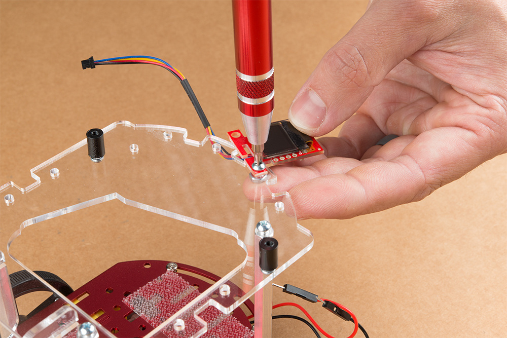
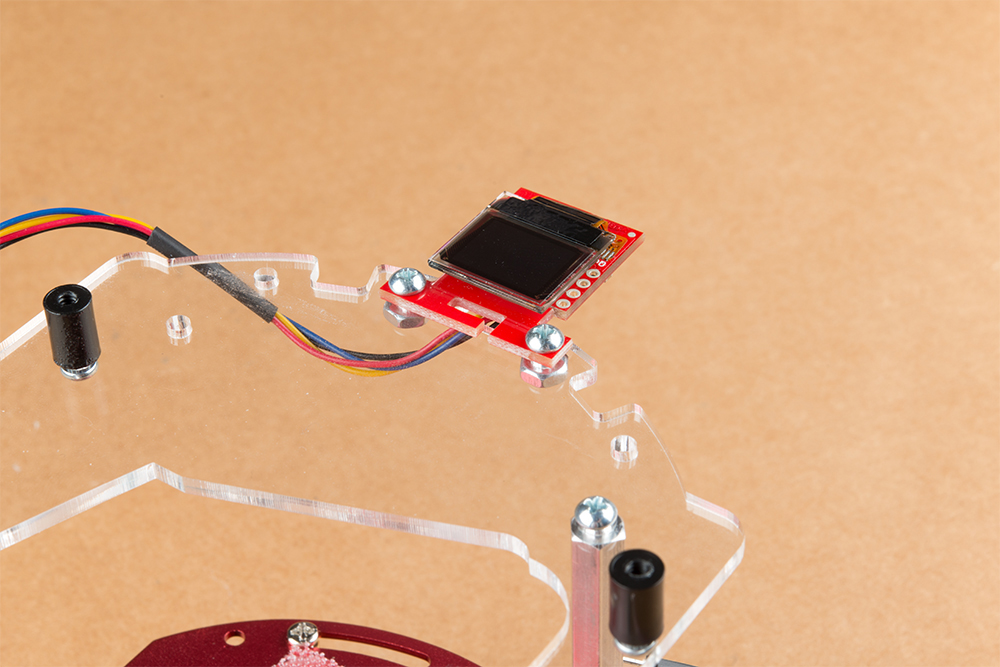
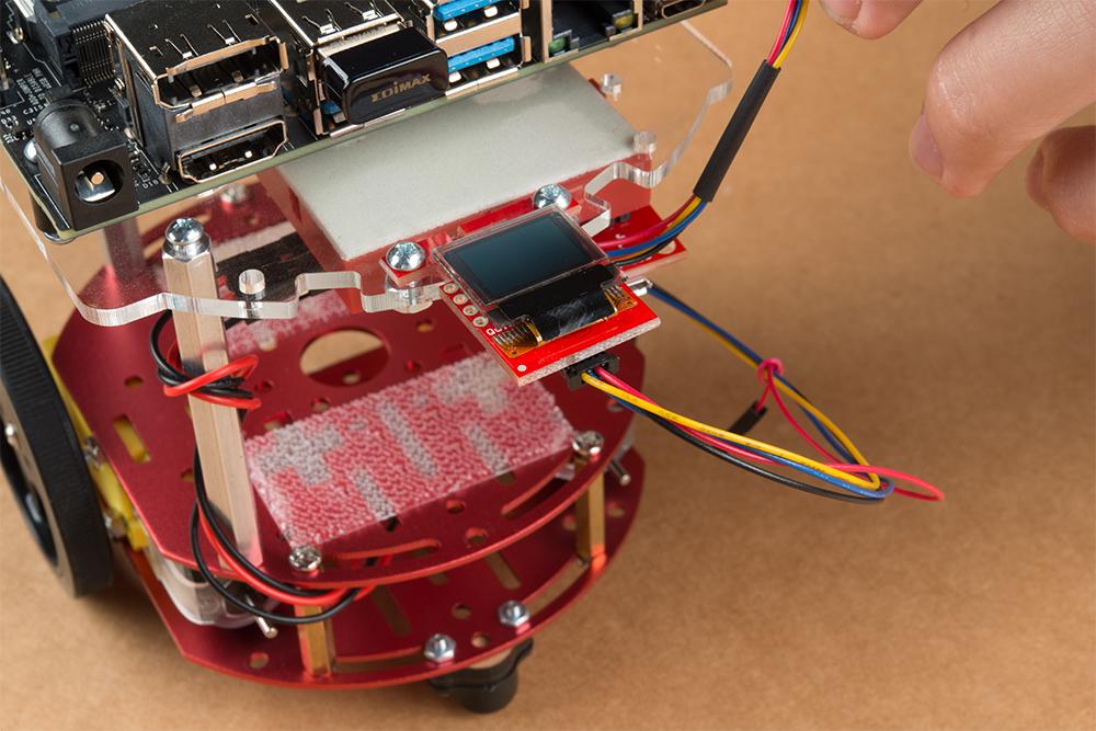
Align the mounting holes on the SparkFun Micro OLED (Qwiic) with those on the back of the SparkFun Jetbot acrylic mounting plate. Install the Micro OLED using two 1/4 in 4-40 Phillips head screws and two 4-40 machine screw nuts.
Thread the ribbon cable of the Leopard imaging camera back through the acrylic mounting plate and half-helix towards the left side of the Jetbot.
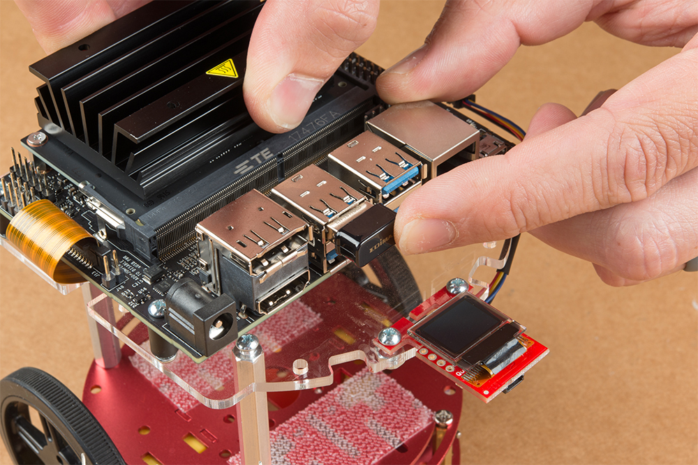
Install the Jetson Nano Dev kit to the nylon standoffs using four 1/4 in 4-40 Phillips head screws. Tighten each screw slightly in a criss-cross pattern to ensure the through holes do not bind during install until finger tight. Make sure you can still access the camera ribbon cable.
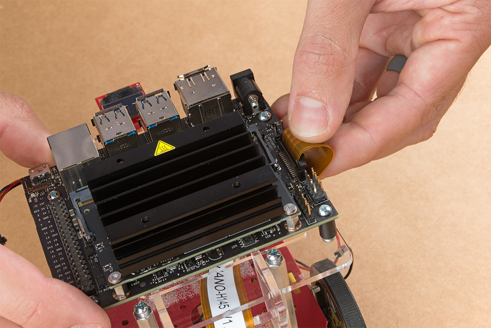
Note: the camera connector is made from small plastic components & can break easier than you think. Please be careful with this next step.
Loosen the camera connector with a fingernail or small flathead screwdriver. Fit the ribbon cable into this connector and depress the plastic press fit piece of the connector to hold the ribbon cable in place.
Unpackage & install the USB Wifi adaptor into one of the USB ports on the Jetson nano Dev Kit. The drivers for this Wifi adaptor are pre-installed on the SparkFun Jetbot image. If you are making your own image, you will need to ensure you get these from Edimax.
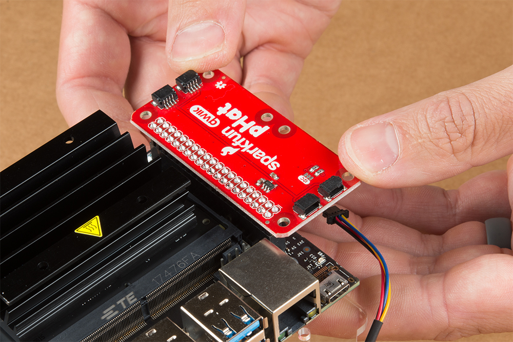
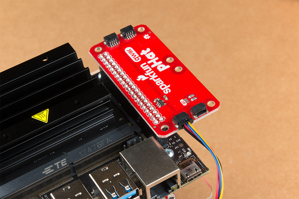
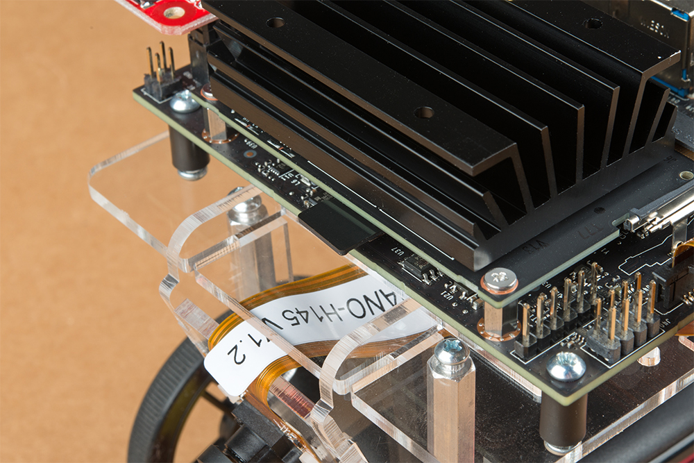
Align the SparkFun pHat with the GPIO headers on the Jetson Nano Dev Kit so that the pHat overhangs the right hand side of the Jetbot. For additional information on hardware assembly of the SparkFun pHat, please reference the hookup guide here.
Note: The heatsink on the Jetson Nano Dev Kit will only allow for one orientation of the SparkFun pHat.
Wrap the motor wires around the rear/left standoff to take up some of the slack; one or two passes should do. Peel the cover off the self adhesive backing on the mini breadboard you set aside at the end of section #3.
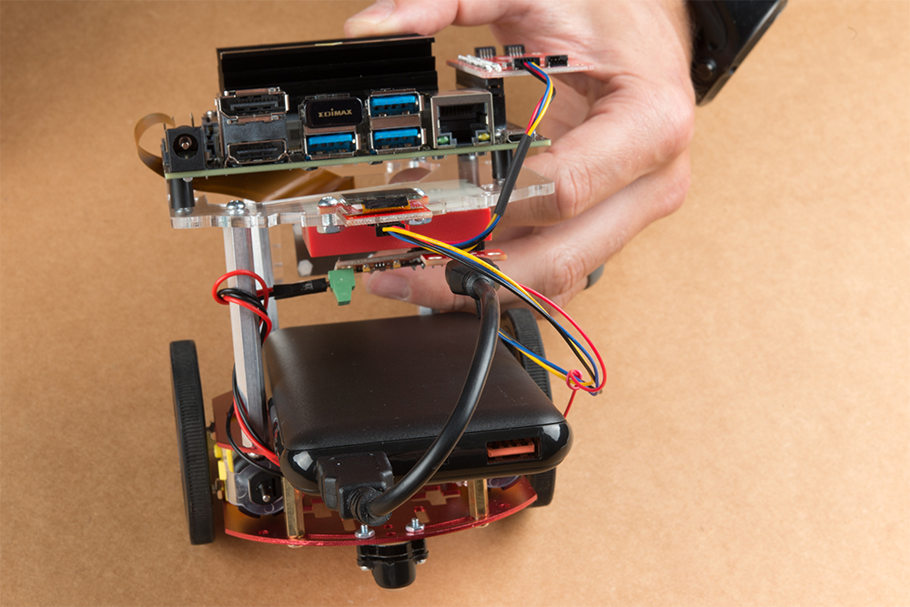
Place the breadboard near the back of the Jetbot Acrylic mounting plate where there is good adhesion & access to all the components. Attach the (4-pin) Female Jumper Qwiic cable to the SparkFun Serial Controlled Motor Driver pins as shown. Yellow to ”SCL,” Blue to ”SDA,” Black to ”GND.”
Daisy chain the polarized Qwiic connector on the other end of the (4-pin) Female Jumper Qwiic cable into the back of the SparkFun Micro OLED (Qwiic).
Using the 100mm Qwiic Cable attach the SparkFun Micro OLED front Qwiic connector to the SparkFun pHat as shown.
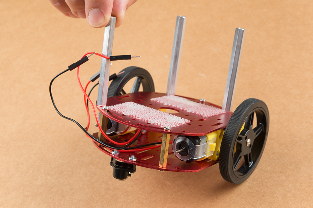
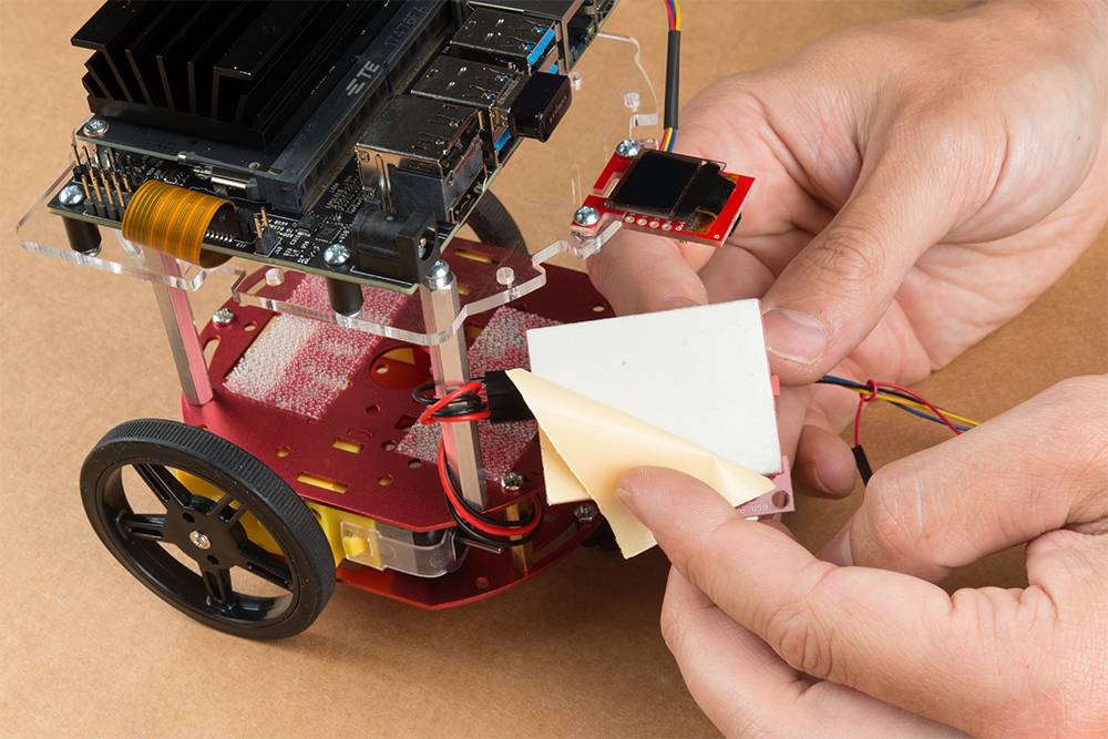
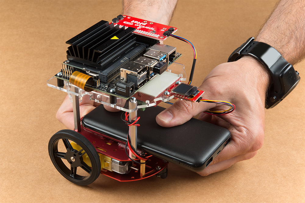
Cut the Dual Lock Velcro into two pieces and align them on the 10Ah battery & top plate of the Two-Layer Circular Robotics Chassis as shown below. Ensure that the USB ports on the battery pack are pointing out the back of the Jetbot. Additionally, the orange port (3A) will need to power the Jetson Nano Dev Kit & therefore will need to be on the right side of the Jetbot.
Apply firm pressure to the battery pack to attach to the Jetbot chassis via the Dual Lock Velcro.
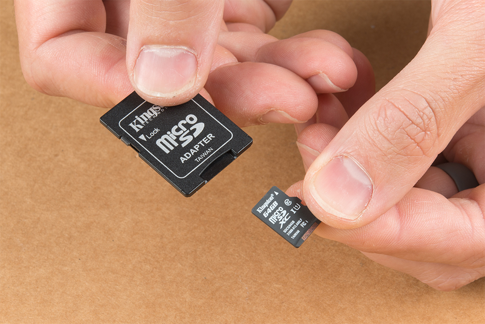
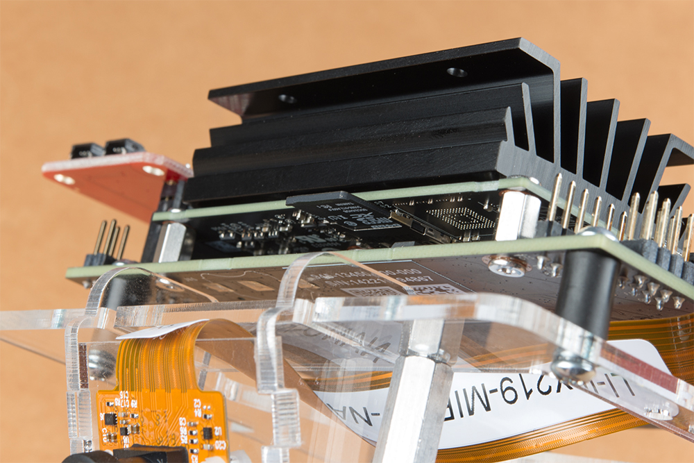
Remove the micro SD card from the SD card adapter.
Insert the micro SD card facing down into the micro SD card slot on the front of the Jetson Nano Dev Kit. Please see the next three pictures for additional details.
The USB ports on the back of the 10Ah battery pack has two differently colored ports. The black port (1A) is used to power the motor driver via the SparkFun microB breakout. Utilize one of the 6 in micro-B USB cables to supply power to the microB breakout.
Note: Once you plug the Jetson Nano Dev Kit into the 3A power port, this will ”Boot Jetson Nano” which is not covered in detail until the links in section #5 of this assembly guide. Do not proceed unless you are ready to move forward with the software setup & examples provided by NVIDIA.
The orange port (3A) is used to power the Jetson Nano Dev Kit. Utilize the remaining 6 in micro-B USB cable to supply power to the Jetson Nano Dev Kit.
Congratulations! You have fully assembled your SparkFun JetBot AI Kit!
5. Software Setup Guide from NVIDIA
Attention: The SD card in this kit comes pre-flashed to work with our hardware and has the all the modules installed (including the sample machine learning models needed for the collision avoidance and object following examples). The only software procedures needed to get your Jetbot running are steps 2-4 from the Nvidia instructions (i.e. setup the WiFi connection and then connect to the Jetbot using a browser). Please DO NOT format or flash a new image on the SD card; otherwise, you will need to flash our image back onto the card (instructions below).
Your SparkFun Jetbot comes with a Pre-Flashed micro SD card. Users only need to plug in the SD card and set up the WiFi connection to get started.
The default password on everything (i.e. login/user, jupyter notebook, and superuser) is ”jetbot”.
We recommend that users change their passwords after initial setup. These are typically covered on the first boot of your Jetson Nano as detailed in the NVIDIA Getting Started with Jetson Nano walkthrough
Software Setup
The only steps needed to get your Jetbot kit up and running is to log into the Jetbot and setup your WiFi connection. Once that is done, you are now ready to connect to the Jetbot wirelessly. If you need instructions for doing so, you can use the link below.However, please take note of our instructions below. You will want to skip steps 1 and 5 to avoid erasing the image on the card or undoing the hardware configuration.NVIDIA JETBOT WIKI SOFTWARE SETUP
Instructions
Skip step 1 of Nvidia’s instructions: It references how to flash your SD card, so feel free to skip to Step 2 – Boot Jetson Nano.
Note: Following Step 1 will erase the pre-flashed image and make a lot of extra work for yourself.
Skip step 5 of Nvidia’s instructions: This step should already be setup on the pre-flashed SD card.
If in the future, you need to update your notebooks, make sure that if you are following Step 5 – Install latest software (optional), skip the last command line instruction of the forth step.
Get and install the latest JetBot repository from GitHub by entering the following commands
COPY CODEgit clone https://github.com/NVIDIA-AI-IOT/jetbot
cd jetbot
sudo python3 setup.py install
Note:Running sudo python3 setup.py install in the command line will overwrite the software modifications for SparkFun’s hardware in the kit.
Troubleshooting
In the event that you accidentally missed the instructions above, here are instructions to get back on track.
Re-Flashing the SD card
If you need to re-flash your SD card, follow the instructions from Step 1 Nvidia’s guide. However, download and use our image instead (click link below).DOWNLOAD SPARKFUN’S JETBOT IMAGENote: Don’t forget to uncompress (i.e. unzip, extract, or expand) the file from the .zip file/folder first. You should be pointing the ”flashing” software to an ~62GB .img file to flash the image (sparkfun_jetbot_v01-00.img) onto the SD card.
Alternatively, there are other options for flashing images onto an SD card. If you have a preferred method, feel free to use the option you are most comfortable with.
Re-Applying the Software Modifications
If you have accidentally, overwritten the software modifications for the hardware included in your kit, you will need to repeat Step 5 from Nvidia’s guide from the desktop interface (if you are comfortable performing the following steps from the command line, feel free to do so).
Skip steps 1 and 2: Plug in a keyboard, mouse, and monitor. Then log in to the desktop interface (if you haven’t changed your password, the default password is: jetbot).
Follow step 3: Launch the terminal. There is an icon on sidebar on the left hand side. Otherwise, you can use the keyboard short cut (Ctrl + Alt + T).
Follow step 4: However, before you execute sudo python3 setup.py install you will want to copy in our file modifications to the jetbot directory you are in.
Begin by downloading our files (click link below).
Next, replace the files in the jetbot folder. The file paths must be the same, so make sure to overwrite files exactly.
Click on the icon that looks like a filing cabinet on the left hand side of the GUI. This is your Home directory. From here, you will need to proceed into the jetbot folder. There you will find a jetbot folder with similar files to the ones you just extracted. Delete the folder and copy in our files (you can also just overwrite the files as well).
Now, you can execute sudo python3 setup.py install in the terminal.
Follow step 5: Finish up by following step 5. Now you are back on track to getting your Jetbot running again!
6. Examples
The ”object following” jupyter notebook example won’t work due to the required dependencies that had not been released by NVIDIA prior to the creation of the SparkFun JetBot image. These updates can be manually installed on your Jetson Nano with the JetPack 4.2.1 release.
Update: The engine generated for the example utilized a previous version of TensorRT and is therefore, not compatible with the latest release. For more details on this issue, check out the following GitHub issue.NVIDIA JETBOT WIKI EXAMPLES
Resources and Going Further
Now that you’ve successfully got your JetBot AI up and running, it’s time to incorporate it into your own project!
For more information, check out the resources below:
Need some inspiration for your next project? Check out some of these related tutorials:
Easy Driver Hook-up Guide
Get started using the SparkFun Easy Driver for those project that need a little motion.
Servo Trigger Hookup Guide
How to use the SparkFun Servo Trigger to control a vast array of Servo Motors, without any programming!
SparkFun 5V/1A LiPo Charger/Booster Hookup Guide
This tutorial shows you how to hook up and use the SparkFun 5V/1A LiPo Charger/Booster circuit.
Wireless Remote Control with micro:bit
In this tutorial, we will utilize the MakeCode radio blocks to have the one micro:bit transmit a signal to a receiving micro:bit on the same channel. Eventually, we will control a micro:bot wirelessly using parts from the arcade:kit!
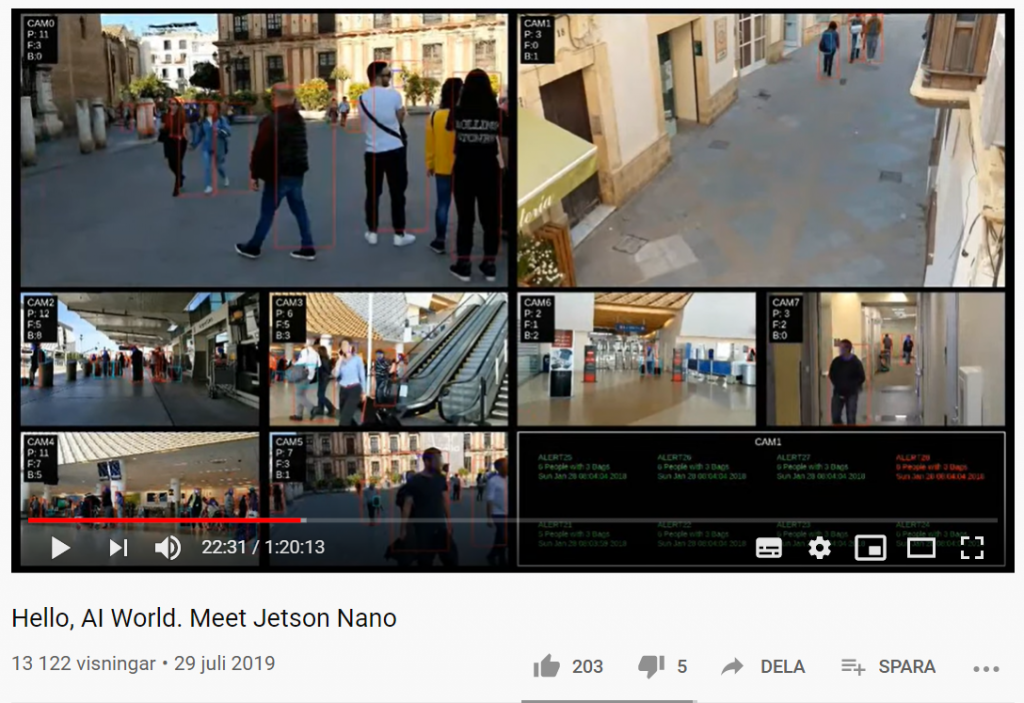
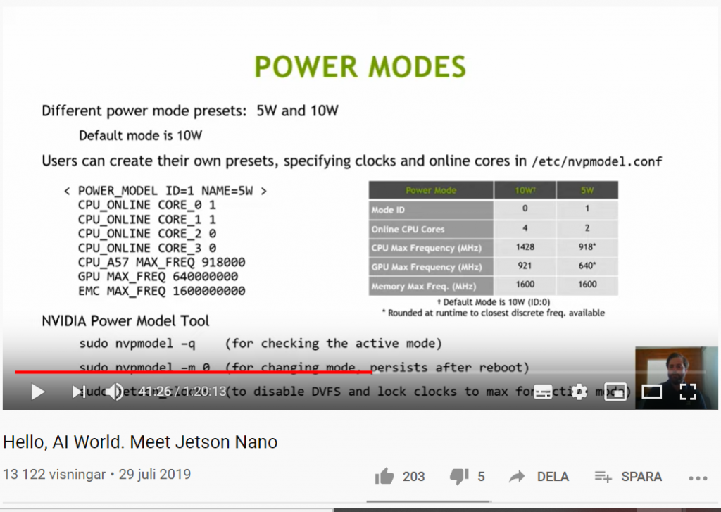
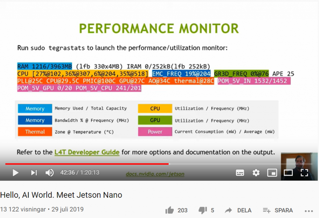
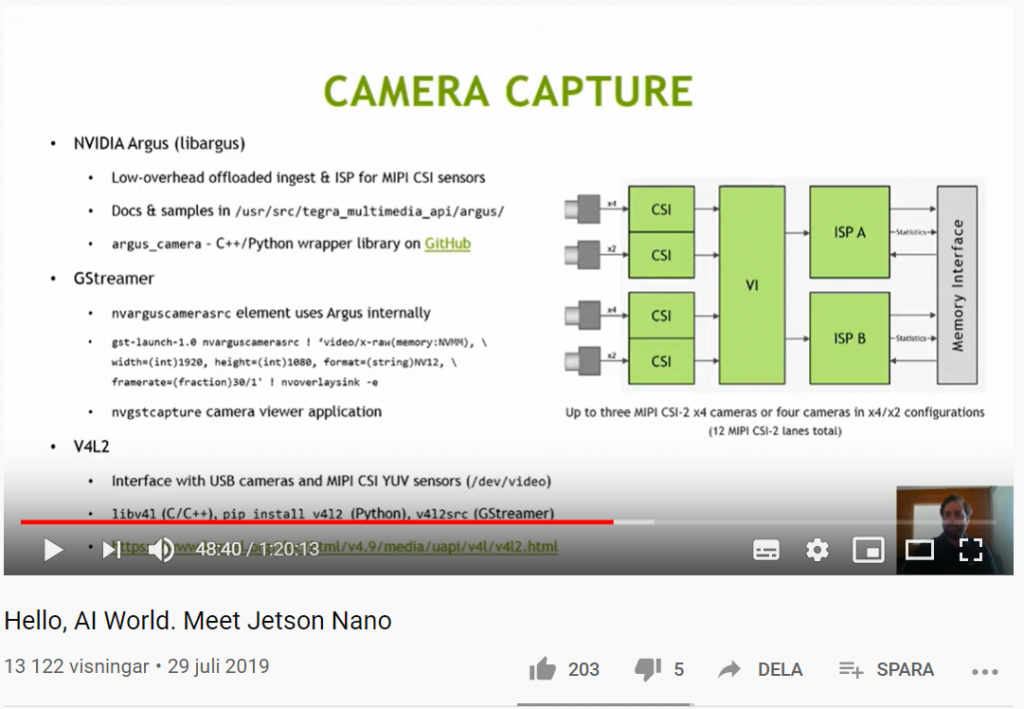
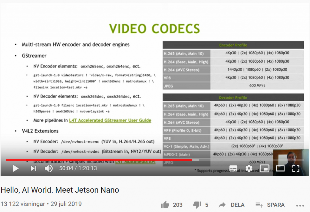
Join us for this engaging, informative webinar and live Q&A session to find out more about the hardware and software behind Jetson Nano. See how you can create and deploy your own deep learning models along with building autonomous robots and smart devices powered by AI. Find more resources for Jetson Nano at https://developer.nvidia.com/embedded…
Här får du möjlighet att bestämma över Sveriges elproduktion. Utmaningen ligger i att ha tillräckligt med effekt när efterfrågan är som störst och att samtidigt hålla koll på miljökonsekvenserna. Du bygger – du bestämmer!
Simulatorn räknar med att tillfälliga överskott exporteras som vid behov importeras senare.
Varje megawatt (MW) elproduktionskapacitet kan bara användas av ett land åt gången. Riktigt kalla dagar skapar ofta brist också i våra grannländer så varje land behöver tillräckligt med kapacitet för att klara effekttoppar.
Räknar ni med energibesparingar?
Vi räknar med dagens elbehov. I framtiden kan behovet av el både öka och minska.
Effektivare användning av elenergi ger ökad ekonomisk konkurrenskraft vilket leder till ekonomisk tillväxt som i sin tur historiskt sett alltid gett högre efterfrågan på el.
Räknar ni med lagring av el?
Vi har inte räknat med lagring av el i nuvarande versionen av Simulatorn.
Ett energilager skapar energiförluster på motsvarande 25 procent vilket gör att mer energi behöver produceras än om ett energilager inte används.
Räknar ni med smarta elnät?
Nej, men införande av smarta elnät ändrar grundläggande inte på våra beräkningar.
Solenergi har ingen tillgänglig effekt?
Tillgänglig effekt i simulatorn beräknas vid tidpunkten då efterfrågan på el är som störst. I Sverige inträffar detta kalla dagar mellan klockan 7-8 på förmiddagen. Eftersom solen inte har gått upp vid denna tidpunkt på vintern kan solpaneler inte producera någon ström då.
Så har vi räknat
Här kommer en beskrivning av hur vi har räknat ut effekt, energi och energiöverskott.
Effekt
Effekten är ett mått på energiproduktionskapaciteten hos en elproduktionsanläggning. Effekten kan delas upp i tre delar.
Installerad effekt
Medeleffekt
Minsta tillgängliga effekt
Installerad effekt (Watt) är helt enkelt den högsta effekt som produktionsanläggningen kan producera. Medeleffekt beräknas genom att ta energiproduktionen (Wh) för en viss period (exempelvis ett år) och dela med antalet timmar för perioden (ett år är 365×24=8760 timmar).
Minsta tillgängliga effekt är den effekt som sannolikt finns tillgängligt vid tidpunkten för den högsta elförbrukningen. I Sverige inträffar den högsta elförbrukningen ungefär klockan 7 på morgonen under kalla vinterdagar.
För att beräkna tillgängligheten för olika kraftslag används Svenska Kraftnäts årliga balansrapport. Det högsta effektbehovet vid en normalvinter är 26 700 MW men vid en s.k. tioårsvinter kan effektbehovet uppgå till 27 700 MW. Tabellen nedan visar prognosen för installerad effekt vid årsskiftet 2019/20 (Svenska Kraftnät). Notera också att vi räknar bort den delen av gaskraften som ingår i störningsreserven (ca 1360 MW):
Kraftslag
Installerad effekt
Tillgänglig effekt
Tillgänglighetsgrad
Vattenkraft
16 318
13 400
82%
Kärnkraft
7 710
6 939
90%
Solkraft
745
0
0%
Vindkraft
9 648
868
11%
Gasturbiner
219
197
90%
Gasturbiner i störningsreserven
1 358
0
0%
Olje-/kolkondens
913
822
90%
Olje-/kolkondens otillgängligt för marknaden
520
0
0%
Mottryck/kraftvärme
4 622
3 536
77%
Mottryck/kraftvärme otillgängligt för marknaden
450
0
0%
Summa
40 503
25 762
–
Kolkraft och solenergi
I våra beräkningar gör vi bedömningen att kolkraft har motsvarande tillgänglighet som kärnkraft och gasturbiner nämligen 90%. För solenergi har vi valt att noll procent finns tillgängligt när effektbehovet vintertid är som störst. I Malmö går solen upp klockan 08:30 och går ner 15:37 vid midvintersolståndet den 21 december. Högst effektbehov uppstår vintertid före åtta och efter sexton då det alltså i hela Sverige fortfarande är mörkt.
Kolkraft, 90% tillgänglig effekt.
Solenergi, 0% tillgänglig effekt.
Svenska Kraftnät räknar med att det under vintern 2019/2020 finns 745 MW installerad solenergi i Sverige.
Beräkning av reglerkraft
När vi beräknar energi så startar vi först med hypotesen att alla anläggningar med låga produktionskostnader körs så mycket som möjligt. All produktion i icke-styrbara produktionsanläggningar som överstiger årsmedelproduktionen antas gå på export. Vind och sol i det nordiska elsystemet är ofta korrelerat så därför går det inte att importera just dessa kraftslag senare i obegränsad omfattning. Begränsningen till medeleffekten bedöms ändå vara generöst tilltaget.
Elbehov minus produktion utan reglerkraft minus export ger alltså behovet av reglerkraft.
Vattenkraften antas kunna användas fullt ut som reglerkraft även om det i genom vattendomar och andra fysiska begränsningar i praktiken inte är möjligt. När vattenkraften inte räcker till kan gasturbiner eller annan reglerkraft köras under begränsad tid. Reservanläggningar som vissa gasturbiner och oljekondenskraftverk beräknas köras i försumbar omfattning. Kärnkraft och kolkraft, när den finns, beräknas köras så många timmar som möjligt (ca 8 000 timmar per år).
Förenklingar
Simulatorn är tänkt att ge en känsla för begreppen installerad effekt, tillgänglig effekt och relationen till total energiproduktion. Vi tar inte hänsyn till följande saker
Överföringsförluster
Begränsningar i elnätet
Begränsningar i vattenkraftens reglerförmåga
Bara delvis tagit hänsyn till begränsningar för import/export
Dessa avgränsningar har gjorts för att göra simulatorn enkel att använda och ge största möjliga förståelse utan avkall på trovärdigheten i det större perspektivet.
Övriga produktionsslag antas ha lågt eller inget fast avfall.
Koldioxid CO2
Alla produktionsslag ger upphov till koldioxidutsläpp vid byggnation, bränsleutvinning, drift, rivning, etc. Utsläpp beräknas enligt livcykelmodellen. I första hand har vi använt Vattenfalls beräkningar och i andra hand valt andra källor. Koldioxidutsläpp i simulatorn beräknas enligt följande tabell
Källa: SMHI Vattenkraft orörda älvar, Potential totalt (TWh) 35 Nyttjande tid (h) 4000 Fördelat på fyra älvar baserat på flöden ger följande potential per älv.
Älv
Flöde (m3/s)
Procent
Energi (TWh)
Effekt (MW)
Torneälven
388
35%
12.4
5 662
Kalixälven
295
27%
9.4
4 292
Piteälven
167
15%
5.3
2 420
Vindelälven
249
23%
7.9
3 607
Summa
1 099
100%
35
15 981
Mer om elnät
Elnät används för att distribuera el från elproducenter till konsumenter. Kostnaden för elnäten beror i huvudsak på två faktorer, avstånd mellan produktion och konsumtion och hur effektivt elledningarna utnyttjas (kapacitetsfaktor).
Ett elnät med korta avstånd mellan produktion och konsumtion ger ett relativt billigare elnät jämfört med ett elnät med långa avstånd.
Långa avstånd ger också betydande överföringsförluster. En tumregel är att 6-10 procent av elen förloras per 1000 km i en 400 kilovolt högspänningsledning.
Enligt världsbanken är de genomsnittliga förluster för svenska elnätet 7 procent eller ungefär 10 TWh vilket är jämförbart med vindkraftens produktion 2013.
Ett elnät med korta avstånd och hög utnyttjandegrad per ledning är därför avgörande för att hålla kostnaderna och överföringsförlusterna så låga som möjligt.
För en vanlig elkund är elnätskostnaderna inte sällan högre än kostnaden för själva elen (elhandelskostnaden).
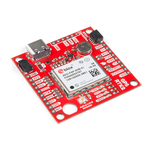
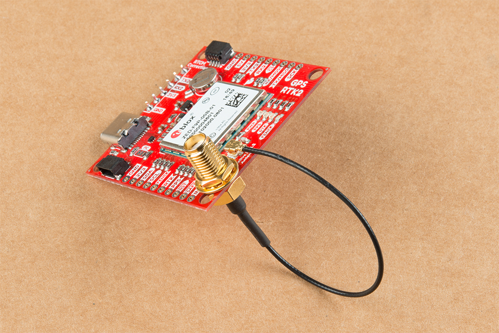
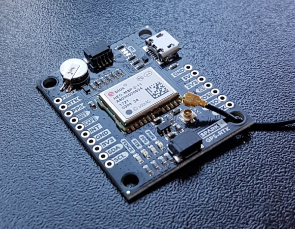
The SparkFun GPS-RTK2 raises the bar for high-precision GPS. Utilizing the latest ZED-F9P module from u-blox the RTK2 is capable of 10mm 3 dimensional accuracy. Yes, you read that right, the SparkFun GPS-RTK2 board can output your X, Y, and Z location that is roughly the width of your fingernail. With great power comes a few requirements: high precision GPS requires a clear view of the sky (sorry, no indoor location) and a stream of correction data from an RTCM source. We’ll get into this more in a later section but as long as you have two GPS-RTK2 units, or access to an online correction source, your GPS-RTK2 can output lat, long, and altitude with centimeter grade accuracy.
An introduction to I2C, one of the main embedded communications protocols in use today.
Serial Basic Hookup Guide
Get connected quickly with this Serial to USB adapter.
What is GPS RTK?
Learn about the latest generation of GPS and GNSS receivers to get 2.5cm positional accuracy!
Getting Started with U-Center for u-blox
Learn the tips and tricks to use the u-blox software tool to configure your GPS receiver.
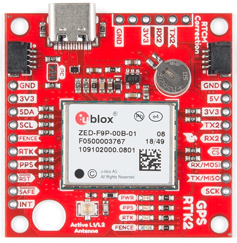
Hardware Overview
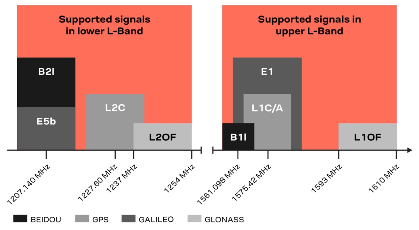
One of the key differentiators between the ZED-F9P and almost all other low-cost RTK solutions is the ZED-F9P is capable of receiving both L1 and L2 bands.
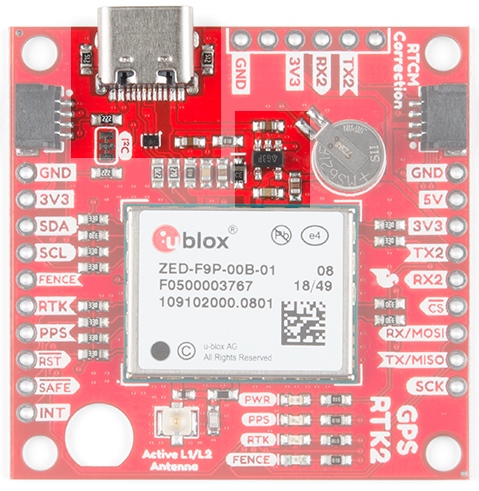
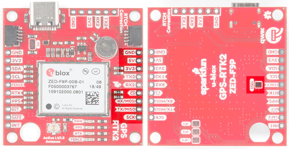
Communication Ports
The ZED-F9P is unique in that it has five communication ports which are all active simultaneously. You can read NMEA data over I2C while you send configuration commands over the UART and vice/versa. The only limit is that the SPI pins are mapped onto the I2C and UART pins so it’s either SPI or I2C+UART. The USB port is available at all times.
USB
The USB C connector makes it easy to connect the ZED-F9P to u-center for configuration and quick viewing of NMEA sentences. It is also possible to connect a Raspberry Pi or other SBC over USB. The ZED-F9P enumerates as a serial COM port and it is a separate serial port from the UART interface. See Getting Started with U-Center for more information about getting the USB port to be a serial COM port.
A 3.3V regulator is provided to regulate the 5V USB down to 3.3V the module requires. External 5V can be applied or a direct feed of 3.3V can be provided. Note that if you’re provide the board with 3.3V directly it should be a clean supply with minimal noise (less than 50mV VPP ripple is ideal for precision locating).
The 3.3V regulator is capable of sourcing 600mA from a 5V input and the USB C connection is capable of sourcing 2A.
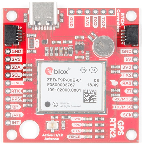
I2C (a.k.a DDC)
The u-blox ZED-F9P has a “DDC” port which is really just an I2C port (without all the fuss of trademark issues). All features are accessible over the I2C ports including reading NMEA sentences, sending UBX configuration strings, piping RTCM data into the module, etc. We’ve written an extensive Arduino library showing how to configure most aspects of the ZED-F9P making I2C our preferred communication method on the ZED. You can get the library through the Arduino library manager by searching ‘SparkFun Ublox’. Checkout the SparkFun U-blox Library section for more information.
The GPS-RTK2 from SparkFun also includes two Qwiic connectors to make daisy chaining this GPS receiver with a large variety of I2C devices. Checkout Qwiic for your next project.
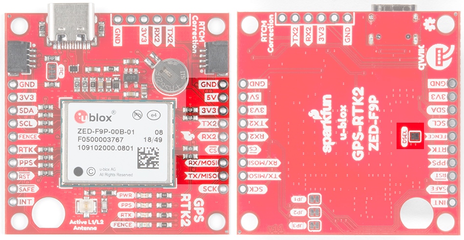
UART/Serial
The classic serial pins are available on the ZED-F9P but are shared with the SPI pins. By default, the UART pins are enabled. Be sure the DSEL jumper on the rear of the board is open.
TX/MISO = TX out from ZED-F9P
RX/MOSI = RX into ZED-F9P
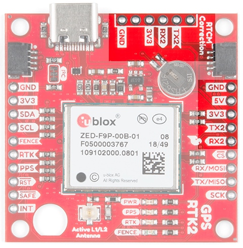
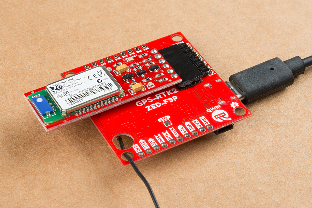
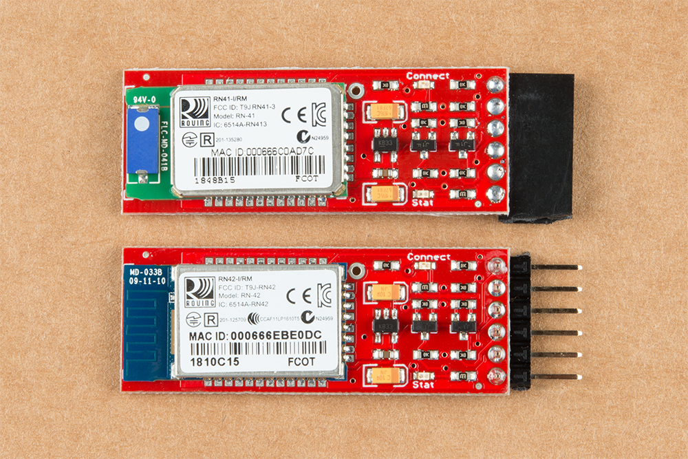
There is a second serial port (UART2) available on the ZED-F9P that is primarily used for RTCM3 correction data. By default, this port will automatically receive and parse incoming RTCM3 strings enabling RTK mode on the board. In addition to the TX2/RX2 pins we have added an additional ‘RTCM Correction’ port where we arranged the pins to match the industry standard serial connection (aka the ’FTDI’ pinout). This pinout is compatible with our Bluetooth Mate and Serial Basic so you can send RTCM correction data from a cell phone or computer. Note that RTCM3 data can also be sent over I2C, UART1, SPI, or USB if desired.
The RTCM correction port (UART2) defaults to 38400bps serial but can be configured via software commands (checkout our Arduino library) or over USB using u-center. Keep in mind our Bluetooth Mate defaults to 115200bps. If you plan to use Bluetooth for correction data (we found it to be easiest), we recommend you increase this port speed to 115200bps using u-center. Additionally, but less often needed, the UART2 can be configured for NMEA output. In general, we don’t use UART2 for anything but RTCM correction data, so we recommend leaving the in/out protocols as RTCM.
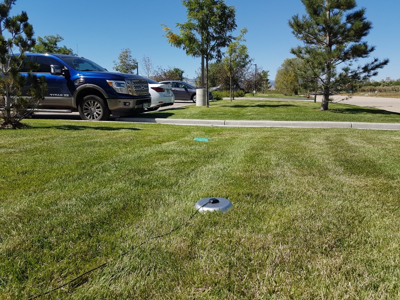
If you’ve got the ZED-F9P setup for base station mode (also called survey-in mode) the UART2 will output RTCM3 correction data. This means you can connect a radio or wired link to UART2 and the board will automatically send just RTCM bytes over the link (no NMEA data taking up bandwidth).
Base station setup to send RTCM bytes out over Bluetooth
SPI
The ZED-F9P can also be configured for SPI communication. By default, the SPI port is disabled. To enable SPI close the DSEL jumper on the rear of the board. Closing this jumper will disable the UART1 and I2C interfaces (UART2 will continue to operate as normal).
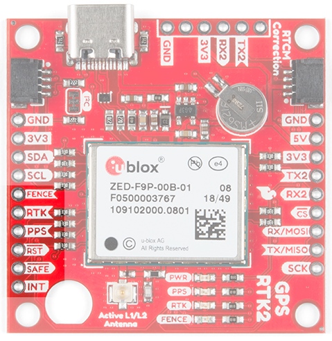
Control Pins
The control pins are highlighted below.
These pins are used for various extra control of the ZED-F9P:
FENCE: Geofence output pin. Configured with U-Center. Will go high or low when a geofence is setup. Useful for triggering alarms and actions when the module exits a programmed perimeter.
RTK: Real Time Kinematic output pin. Remains high when module is in normal GPS mode. Begins blinking when RTCM corrections are received and module enters RTK float mode. Goes low when module enters RTK fixed mode and begins outputting cm-level accurate locations.
PPS: Pulse-per-second output pin. Begins blinking at 1Hz when module gets basic GPS/GNSS position lock.
RST: Reset input pin. Pull this line low to reset the module.
SAFE: Safeboot input pin. This is required for firmware updates to the module and generally should not be used or connected.
INT: Interrupt input/output pin. Can be configured using U-Center to bring the module out of deep sleep or to output an interrupt for various module states.
Antenna
The ZED-F9P requires a good quality GPS or GNSS (preferred) antenna. A U.FL connector is provided. Note: U.FL connectors are rated for only a few mating cycles (about 30) so we recommend you set it and forget it. A U.FL to SMA cable threaded through the mounting hole provides a robust connection that is also easy to disconnect at the SMA connection if needed. Low-cost magnetic GPS/GNSS antennas can be used (checkout the ublox white paper) but a 4” / 10cm metal disc is required to be placed under the antenna as a ground plane.
A cutout for the SMA bulkhead is available for those who want an extra sturdy connection. We recommended installing the SMA into the board only when the board is mounted in an enclosure. Otherwise, the cable runs the risk of being damaged when compressed (for example, students carrying the board loose in a backpack).
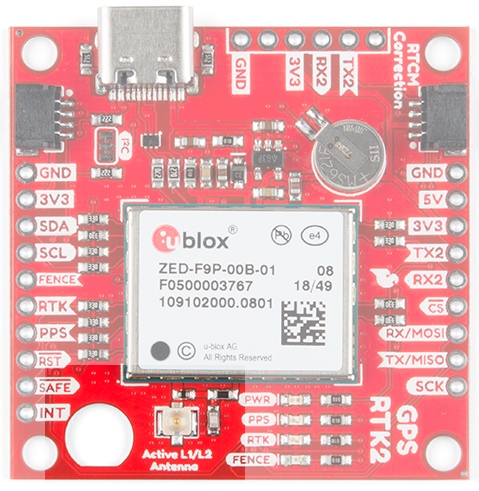
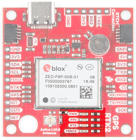
LEDs
The board includes four status LEDs as indicated in the image below.
PWR: The power LED will illuminate when 3.3V is activated either over USB or via the Qwiic bus.
PPS: The pulse per second LED will illuminate each second once a position lock has been achieved.
RTK: The RTK LED will be illuminated constantly upon power up. Once RTCM data has been successfully received it will begin to blink. This is a good way to see if the ZED-F9P is getting RTCM from various sources. Once an RTK fix is obtained, the LED will turn off.
FENCE: The FENCE LED can be configured to turn on/off for geofencing applications.
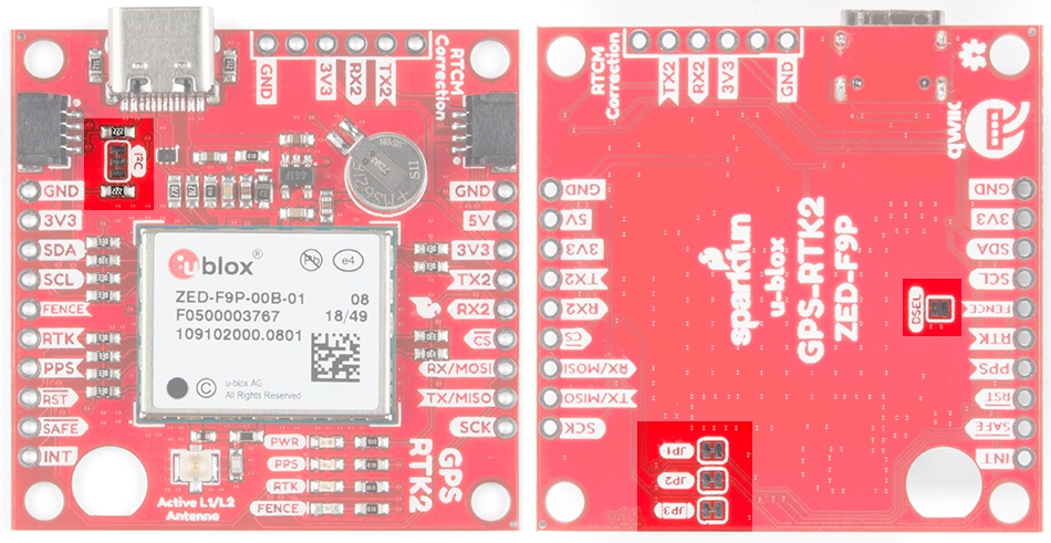
Jumpers
There are five jumpers used to configure the GPS-RTK2.
Closing DSEL with solder enables the SPI interface and disables the UART and I2C interfaces. USB will still function.
Cutting the I2C jumper will remove the 2.2k Ohm resistors from the I2C bus. If you have many devices on your I2C bus you may want to remove these jumpers. Not sure how to cut a jumper? Read here!
Cutting the JP1, JP2, JP3 jumpers will disconnect of the various status LEDs from their associated pins.
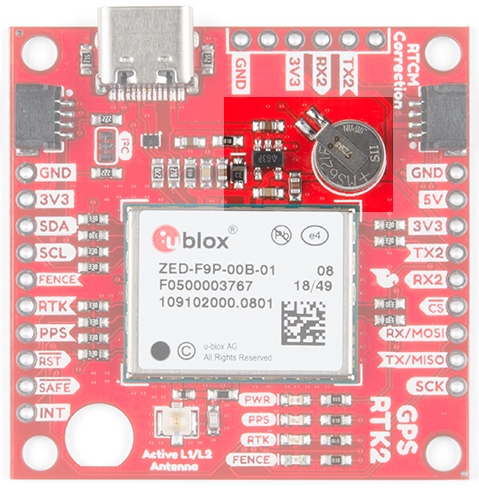
Backup Battery
The MS621FE rechargeable battery maintains the battery backed RAM (BBR) on the GNSS module. This allows for much faster position locks. The BBR is also used for module configuration retention. The battery is automatically trickle charged when power is applied and should maintain settings and GNSS orbit data for up to two weeks without power.
Connecting an Antenna
U.FL connectors are very good but they are a designed to be implemented inside a small embedded application like a laptop. Exposing a U.FL connector to the wild risks it getting damaged. To prevent damaging the U.FL connection we recommend threading the U.FL cable through the stand-off hole, then attach the U.FL connectors. This will provide a great stress relief for the antenna connection. Now attach your SMA antenna of choice.
Be Careful! U.FL connectors are easily damaged. Make sure the connectors are aligned, flush face to face (not at an angle), then press down using a rigid blunt edge such as the edge of a PCB or point of a small flat head screwdriver. For more information checkout our tutorial Three Quick Tips About Using U.FL.
Three Quick Tips About Using U.FL
DECEMBER 28, 2018
Quick tips regarding how to connect, protect, and disconnect U.FL connectors.
Additionally, a bulkhead cut-out is provided to screw the SMA onto the PCB if desired.
While this method decreases stress from the U.FL connector it is only recommended when the board has been permanently mounted. If the board is not mounted, the cable on the U.FL cable is susceptible to being kinked causing impedance changes that may decrease reception quality.
If you’re indoors you must run a SMA extension cable long enough to locate the antenna where it has a clear view of the sky. That means no trees, buildings, walls, vehicles, or concrete metally things between the antenna and the sky. Be sure to mount the antenna on a 4”/10cm metal ground plate to increase reception.
Connecting the GPS-RTK2 to a Correction Source
Before you go out into the field it’s good to understand how to get RTCM data and how to pipe it to the GPS-RTK2. We recommend you read Connecting a Correction Source section of the original GPS-RTK tutorial. This will give you the basics of how to get a UNAVCO account and how to identify a Mount Point within 10km of where your ZED-F9P rover will be used. This section builds upon these concepts.
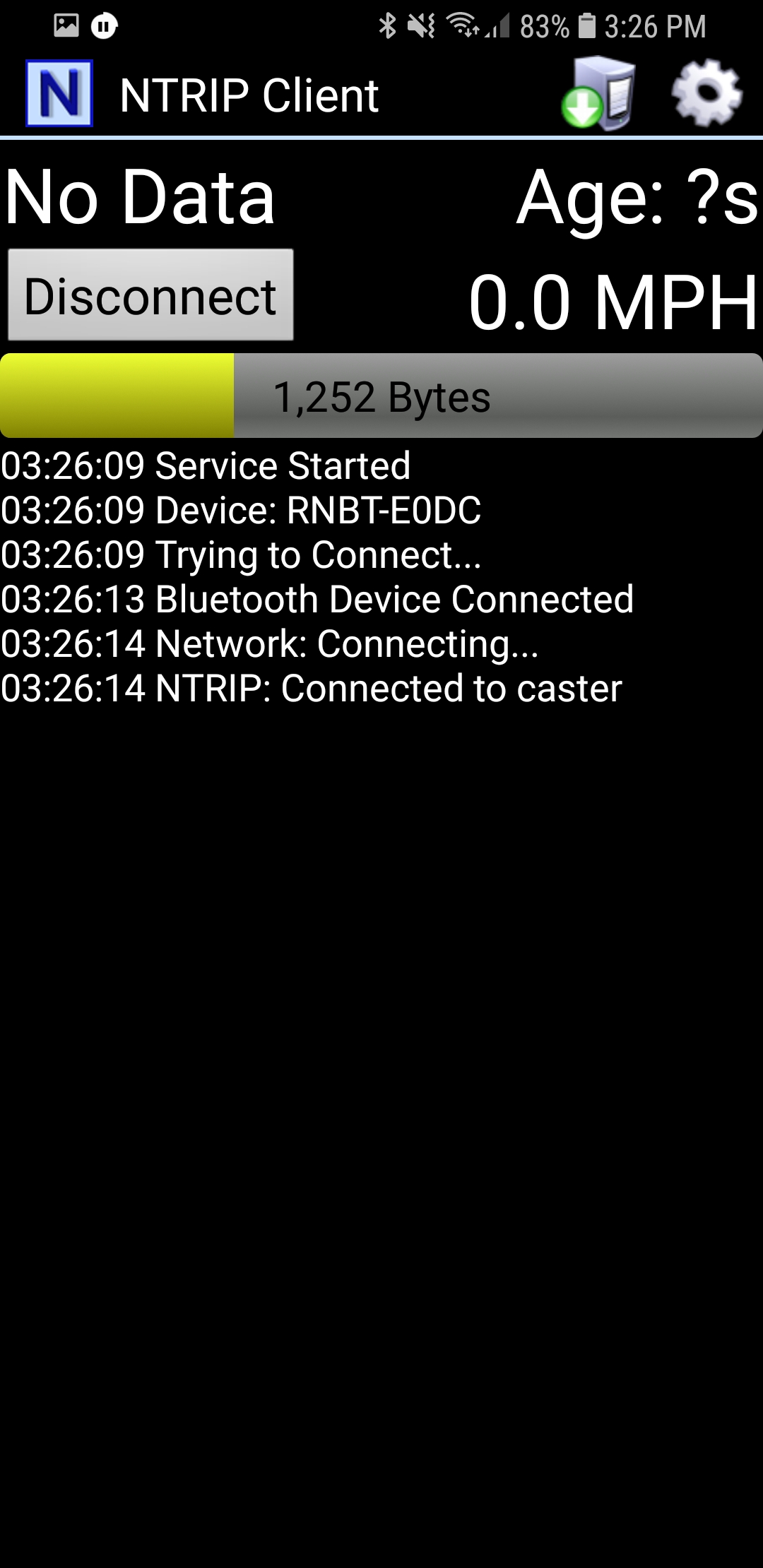
For this example, we will show how to get correction data from the UNAVCO network and pull that data in using the Android app called NTRIP Client. The correction data will then be transmitted from the app over Bluetooth to the ZED-F9P using the SparkFun Bluetooth Mate.
Get the NTRIP By Lefebure app from Google Play. There seem to be NTRIP apps for iOS but we have not been able to verify any one app in particular. If you have a favorite, please let us know.
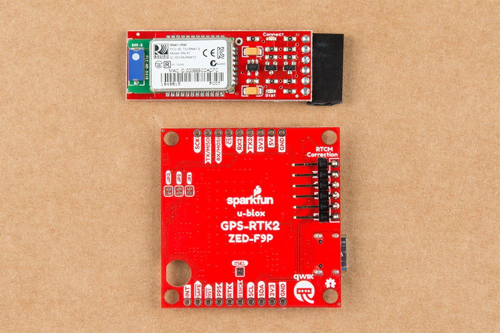
First we need to attach the Bluetooth Module to the GPS-RTK2 board. Solder a female header to the Bluetooth Mate so that it hangs off the end.
On the GPS-RTK2 board we recommend soldering the right-angle male header underneath the board. This will allow the Bluetooth module to be succinctly tucked under the board.
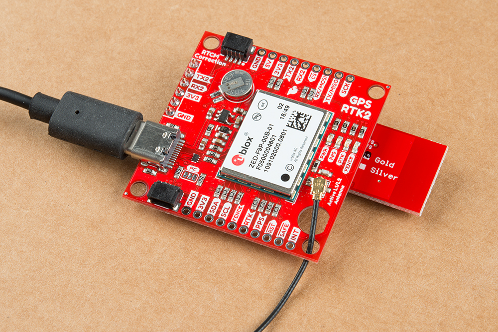
When attaching the Bluetooth Mate to GPS-RTK2 be sure to align the pins so that the GND indicator align on both Bluetooth module and RTK board. Once Bluetooth has been installed attach your GNSS antenna and connect the RTK2 board over USB. This will power the board and the Bluetooth Mate.
Where the male and female headers go is personal preference. For example, here are two Bluetooth Mates; one with male headers, one with female.
Soldering a female header to a Bluetooth Mate makes it easier to add Bluetooth to boards that have a ’FTDI’ style connection like our OpenScale, Arduino Pro, or Simultaneous RFID Reader. Whereas, soldering a male header to the Bluetooth Mate makes it much easier to use in a breadboard. It’s really up to you!
The Bluetooth Mate defaults to 115200bps whereas the RTK2 is expecting serial over UART2 to be 38400bps. To fix this we need to open u-center and change the port settings for UART2. If you haven’t already, be sure to checkout the tutorial Getting Started with U-Center to get your bearings.
Open the Configure window and navigate to the PRT (Ports) section. Drop down the target to UART2 and set the baud rate to 115200. Finally, click on the ‘Send’ button.
By this time you should have a valid 3D GPS lock with ~1.5m accuracy. It’s about to get a lot better.
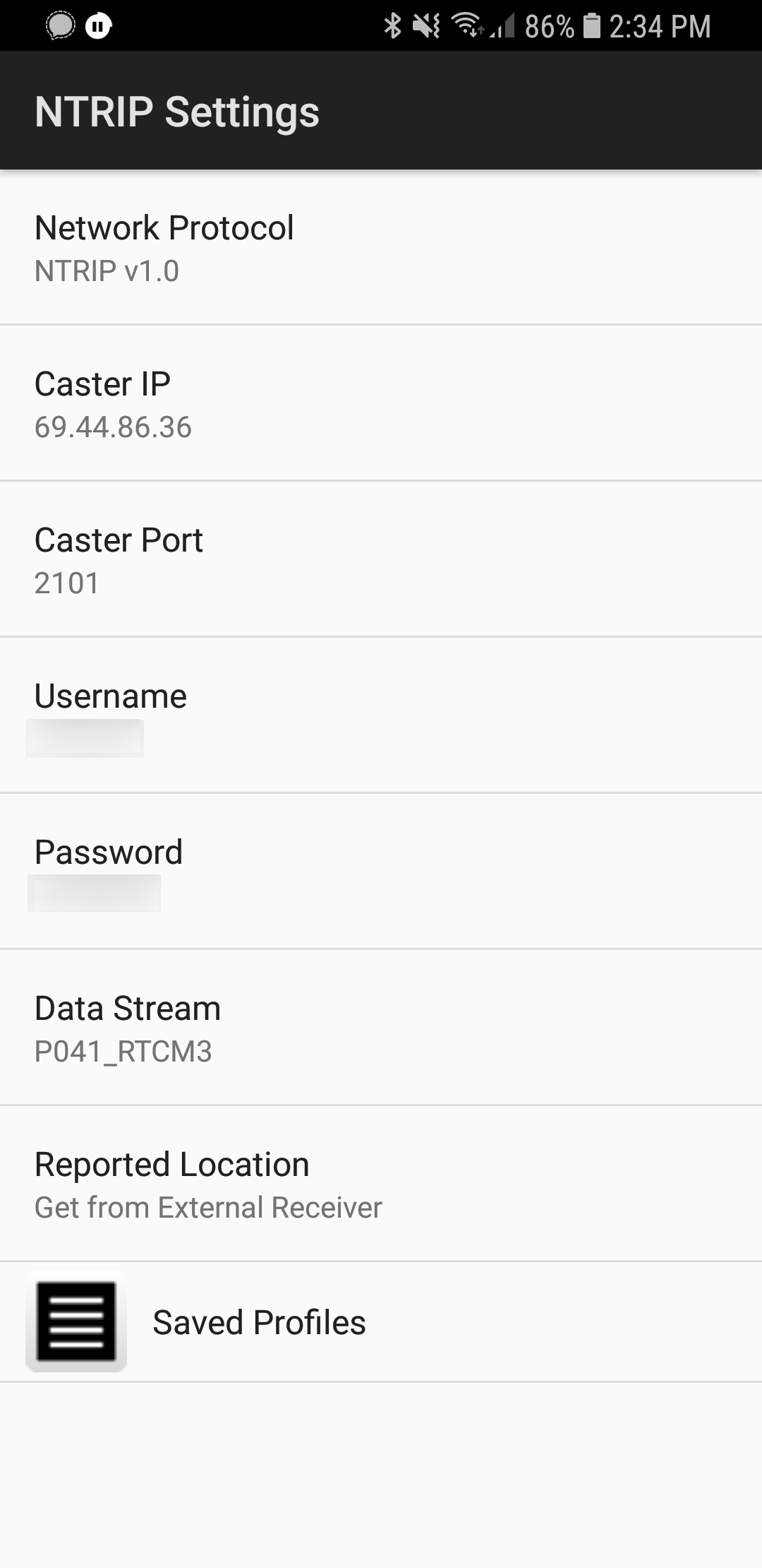
We are going to assume you’ve read the original RTK tutorial and obtained your UNAVCO credentials including the following:
Username
Password
IP Address for UNAVCO (69.44.86.36 at time of writing)
Caster Port (2101 at time of writing)
Data Stream a.k.a. Mount Point (‘P041_RTCM3’ if you want the one near Boulder, CO – but you should really find one nearest your rover location)
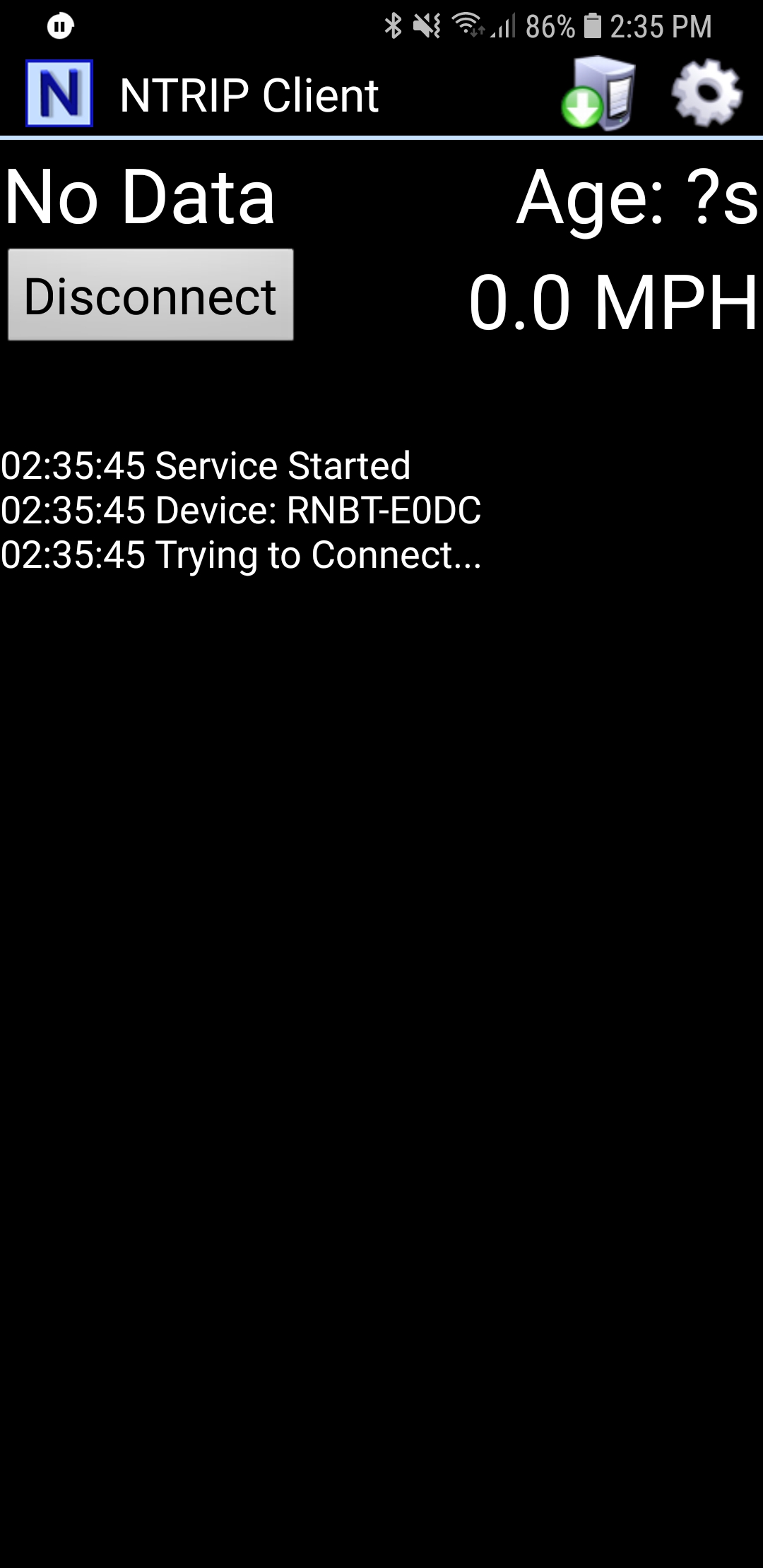
The Bluetooth Mate should be powered up. From your phone, discover the Bluetooth Mate and pair with it. The module used in this tutorial was discovered as RNBT-E0DC where E0DC is the last four characters of the MAC address of the module and should be unique to your module.
Once you have your UNAVCO credentials and you’ve paired with the Bluetooth module open the NTRIP client.
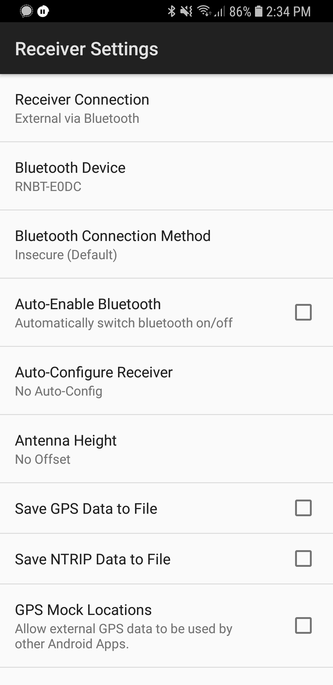
From the home screen, click on the gear in upper right corner then Receiver Settings.
Verify that the Receiver Connection is set to Bluetooth then select Bluetooth Device and select the Bluetooth module you just paired with. Next, open NTRIP settings and enter your credentials including mounting point (a.k.a. Data Stream).
This example demonstrates how to obtain correction data from UNAVCO’s servers but you could similarly setup your own base station using another ZED-F9P and RTKLIB to broadcast the correction data. This NTRIP app would connect to your RTKLIB based server giving you some amazing flexibility (the base station could be anywhere there’s a laptop and Wifi within 10km of your rover).
Ok. You ready? This is the fun part. Return to the main NTRIP window and click Connect. The app will connect to the Bluetooth module. Once connected, it will then connect to your NTRIP source. Once data is flowing you will see the number of bytes increase every second.
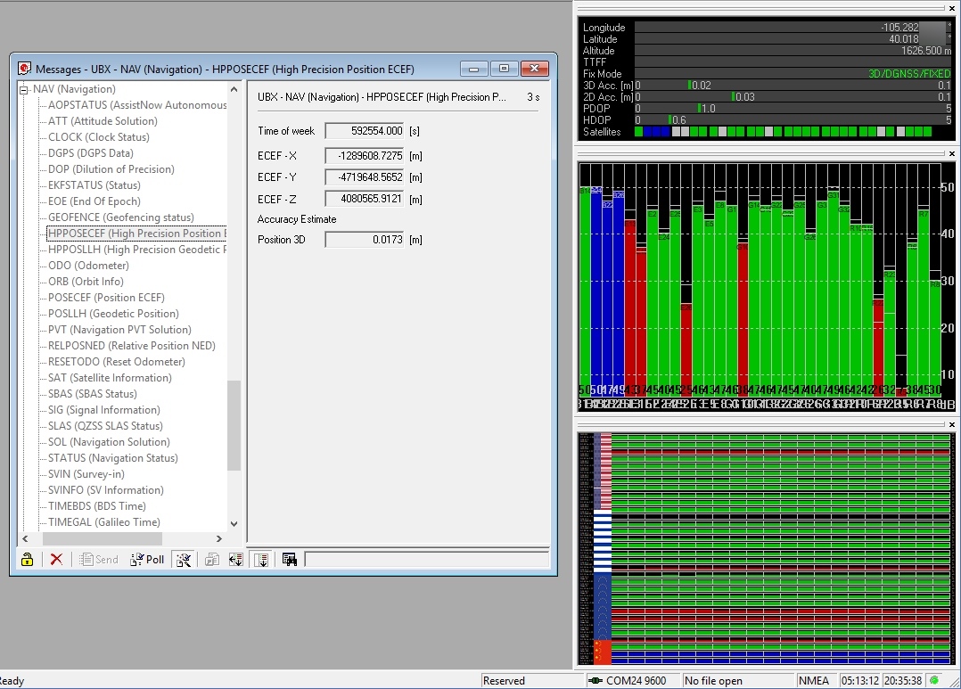
Within a few seconds you should see the RTK LED on the GPS-RTK2 board turn off. This indicates you have an RTK fix. To verify this, open u-center on your computer. The first thing to notice is that Fix Mode in the left hand black window has changed from 3D to 3D/DGNSS/FIXED.
Navigate to the UBX-NAV-HPPOSECEF message. This will show you a high-precision 3D accuracy estimate. We were able to achieve 17mm accuracy using a low-cost GNSS antenna with a metal plate ground plane and we were over 10km from the correction station.
Congrats! You now know where you are within the diameter of a dime!
SparkFun U-blox Library
Note: This example assumes you are using the latest version of the Arduino IDE on your desktop. If this is your first time using Arduino, please review our tutorial on installing the Arduino IDE. If you have not previously installed an Arduino library, please check out our installation guide.
The SparkFun Ublox Arduino library enables the reading of all positional datums as well as sending binary UBX configuration commands over I2C. This is helpful for configuring advanced modules like the ZED-F9P but also the NEO-M8P-2, SAM-M8Q and any other Ublox module that use the Ublox binary protocol.
Once you have the library installed checkout the various examples.
Example1: Read NMEA sentences over I2C using Ublox module SAM-M8Q, NEO-M8P, etc
Example2: Parse NMEA sentences using MicroNMEA library. This example also demonstrates how to overwrite the processNMEA function so that you can direct the incoming NMEA characters from the Ublox module to any library, display, radio, etc that you prefer.
Example3: Get latitude, longitude, altitude, and satellites in view (SIV). This example also demonstrates how to turn off NMEA messages being sent out of the I2C port. You’ll still see NMEA on UART1 and USB, but not on I2C. Using only UBX binary messages helps reduce I2C traffic and is a much lighter weight protocol.
Example4: Displays what type of a fix you have the two most common being none and a full 3D fix. This sketch also shows how to find out if you have an RTK fix and what type (floating vs. fixed).
Example5: Shows how to get the current speed, heading, and dilution of precision.
Example6: Demonstrates how to increase the output rate from the default 1 per second to many per second; up to 30Hz on some modules!
Example7: Older modules like the SAM-M8Q utilize an older protocol (version 18) whereas the newer modules like the ZED-F9P depricate some commands using the latest protocol (version 27). This sketch shows how to query the module to get the protocol version.
Example8: Ublox modules use I2C address 0x42 but this is configurable via software. This sketch will allow you to change the module’s I2C address.
Example9: Altitude is not a simple measurement. This sketch shows how to get both the ellipsoid based altitude and the MSL (mean sea level) based altitude readings.
Example10: Sometimes you just need to do a hard reset of the hardware. This sketch shows how to set your Ublox module back to factory default settings.
NEO-M8P
NEO-M8P Example1: Send UBX binary commands to enable RTCM sentences on U-blox NEO-M8P-2 module. This example is one of the steps required to setup the NEO-M8P as a base station. For more information have a look at the Ublox manual for setting up an RTK link.
NEO-M8P Example2: This example extends the previous example sending all the commands to the NEO-M8P-2 to have it operate as a base. Additionally the processRTCM function is exposed. This allows the user to overwrite the function to direct the RTCM bytes to whatever connection the user would like (radio, serial, etc).
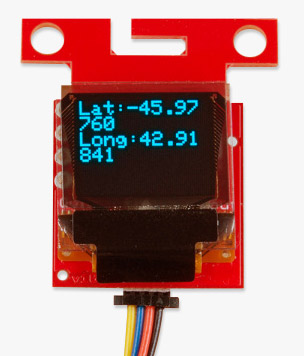
NEO-M8P Example3: This is the same example as NEO-M8P’s Example2. However, the data is sent to a serial LCD via I2C.
ZED-F9P
ZED-F9P Example1: This module is capable of high precision solutions. This sketch shows how to inspect the accuracy of the solution. It’s fun to watch our location accuracy drop into the millimeter scale.
ZED-F9P Example2: The ZED-F9P uses a new Ublox configuration system of VALGET/VALSET/VALDEL. This sketch demonstrates the basics of these methods.
ZED-F9P Example3: Setting up the ZED-F9P as a base station and outputting RTCM data.
ZED-F9P Example4: This is the same example as ZED-F9P’s Example3. However, the data is sent to a serial LCD via I2C.
This SparkFun Ublox library really focuses on I2C because it’s faster than serial and supports daisy-chaining. The library also uses the UBX protocol because it requires far less overhead than NMEA parsing and does not have the precision limitations that NMEA has.
Setting the GPS-RTK2 as a Correction Source
If you’re located further than 20km from a correction station you can create your own station using the ZED-F9P. Ublox provides a setup guide within the ZED-F9P Integration Manual showing the various settings needed via U-Center. We’ll be covering how to setup the GPS-RTK2 using I2C commands only. This will enable a headless (computerless) configuration of a base station that outputs RTCM correction data.
Before getting started we recommend you configure the module using U-Center. Checkout our tutorial on using U-Center then read section 3.5.8 Base Station Configuration of the Ublox Integration Manual for getting the ZED-F9P configured for RTK using U-Center. Once you’ve been successful controlling the module in the comfort of your lab using U-Center, then consider heading outdoors.
For this exercise we’ll be using the following parts:
A 20+ft SMA extension can be handy when first experimenting with base stations so you can sit indoors with a laptop and analyze the output of the GPS-RTK
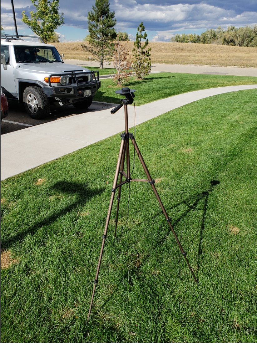
A standard camera tripod
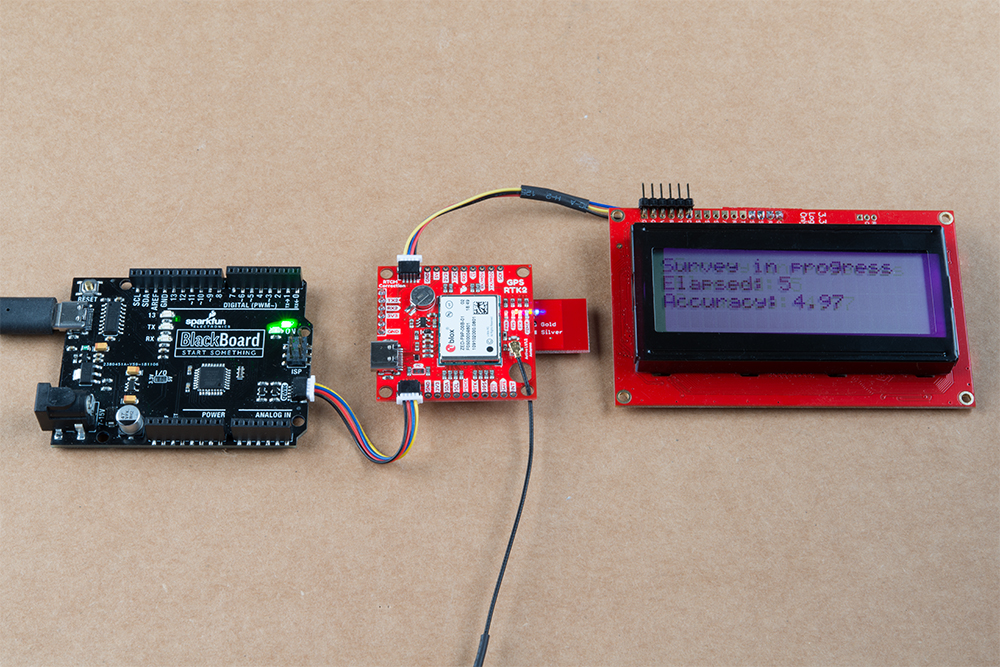
The ZED-F9P can be configured using Serial, SPI, or I2C. We’re fans of the daisychain-ability of I2C so we’ll be focusing on the Qwiic system. For this exercise we’ll be connecting the an LCD and GPS-RTK2 to a BlackBoard using two Qwiic cables.
For the antenna, you’ll need a clear view of the sky. The better your antenna position the better your accuracy and performance of the system. We designed the GPS Antenna Ground Plate to make this setup easy. The plate has a ¼” threaded hole that threads directly onto a camera tripod. The plate thickness was chosen to be thick enough so that the threaded screw is flush with the plate so it won’t interfere with the antenna. Not sure why we’re using a ground plate? Read the Ublox white paper on using low-cost GNSS antennas with RTK. Mount your magnetic mount antenna and run the SMA cable to the U.FL to SMA cable to the GPS-RTK2 board.
There are only three steps to initiating a base station:
Enable Survey-In mode for 1 minute (60 seconds)
Enable RTCM output messages
Being Transmitting the RTCM packets over the backhaul of choice
Be sure to grab the SparkFun Arduino Library for Ublox. You can easily install this via the library manager by searching ‘SparkFun Ublox’. Once installed click on File->Examples->SparkFun_Ublox_Arduino_Library.
The ZED-F9P subfolder houses a handful of sketches specific to its setup. Example3 of the library demonstrates how to send the various commands to the GPS-RTK2 to enable Survey-In mode. Let’s discuss the important bits of code.
The library is capable of sending UBX binary commands with all necessary headers, packet length, and CRC bytes over I2C. The enableSurveyMode(minimumTime, minimumRadius) command does all the hard work to tell the module to go into survey mode. The module will begin to record lock data and calculate a 3D standard deviation. The survey-in process ends when both the minimum time and minimum radius are achieved. Ublox recommends 60 seconds and a radius of 5m. With a clear view of the sky, with a low cost GNSS antenna mounted to a ground plate we’ve seen the survey complete at 61 seconds with a radius of around 1.5m.
COPY CODEresponse &= myGPS.enableRTCMmessage(UBX_RTCM_1005, COM_PORT_I2C, 1); //Enable message 1005 to output through I2C port, message every second
response &= myGPS.enableRTCMmessage(UBX_RTCM_1074, COM_PORT_I2C, 1);
response &= myGPS.enableRTCMmessage(UBX_RTCM_1084, COM_PORT_I2C, 1);
response &= myGPS.enableRTCMmessage(UBX_RTCM_1094, COM_PORT_I2C, 1);
response &= myGPS.enableRTCMmessage(UBX_RTCM_1124, COM_PORT_I2C, 1);
response &= myGPS.enableRTCMmessage(UBX_RTCM_1230, COM_PORT_I2C, 10); //Enable message every 10 seconds
These six lines enable the six RTCM output messages needed for a second GPS-RTK2 to receive correction data. Once these sentences have been enabled (and assuming a survey process is complete) the GPS-RTK2 base module will begin outputting RTCM data every second after the NMEA sentences (the RTCM_1230 sentence will be output once every 10 seconds). You can view an example of what this output looks like here.
The size of the RTCM correction data varies but in general it is approximately 2000 bytes every second (~2500 bytes every 10th second when 1230 is transmitted).
COPY CODE//This function gets called from the SparkFun Ublox Arduino Library.
//As each RTCM byte comes in you can specify what to do with it
//Useful for passing the RTCM correction data to a radio, Ntrip broadcaster, etc.
void SFE_UBLOX_GPS::processRTCM(uint8_t incoming)
{
  //Let's just pretty-print the HEX values for now
  if (myGPS.rtcmFrameCounter % 16 == 0) Serial.println();
  Serial.print(" ");
  if (incoming < 0x10) Serial.print("0");
  Serial.print(incoming, HEX);
}
If you have a ‘rover’ in the field in need of correction data you’ll need to get the RTCM bytes to the rover. The SparkFun Ublox library automatically detects the difference between NMEA sentences and RTCM data. The processRTCM() function allows you to ‘pipe’ just the RTCM correction data to the channel of your choice. Once the base station has completed the survey and has the RTCM messages enabled, your custom processRTCM() function can pass each byte to any number of channels:
Posting the bytes over the internet using WiFi or wired ethernet over an Ntrip caster
Over a wired solution such as RS485
The power of the processRTCM() function is that it doesn’t care; it presents the user with the incoming byte and is agnostic about the back channel.Heads up! We’ve been experimenting with various LoRa solutions and the bandwidth needed for the best RTCM (~500 bytes per second) is right at the usable byte limit for many LoRa setups. It’s possible but you may need to adjust your LoRa settings to reach the throughput necessary for RTK.
What about configuring the rover? Ublox designed the ZED-F9P to automatically go into RTK mode once RTCM data is detected on any of the ports. Simply push the RTCM bytes from your back channel into one of the ports (UART, SPI, I2C) on the rover’s GPS-RTK2 and the location accuracy will go from meters to centimeters. The rover’s NMEA messages will contain the improved Lat/Long data and you’ll know where you are with mind-bending accuracy. It’s a lot of fun to watch!
Can I Really Use NMEA with a High Precision GPS Receiver?
Yes! Except that NMEA sentences are right on the edge of enough precision. NMEA sentences look something like this:
NMEA outputs coordinates in the ddmm.mmmmm format. So what is the weight of the least significant digit? Said differently, what is the impact of one digit change?
COPY CODE104 16.95542
vs
COPY CODE104 16.95543
If we know 1 degree of latitude is 111.3km at the equator, we can glean the change of a fraction of a minute:
1 degree = 60 minutes
1 minute = 1 degree/60 = 111.32km / 60 = 1.855km
1 minute = 1855m
0.1min = 185.5m
0.01min = 18.55m
0.001min = 1.855m
0.0001min = .1855m = 185.5mm
0.00001min = 0.0185m = 18.55mm = 1.855cm
Using the NMEA sentence, the ZED-F9P will only be able to communicate a change of ~1.5cm location change for each digit in the 5th position. This is pretty close to the 1.0cm accuracy of the module. If you want additional precision, you should consider using the UBX protocol which can output up to 8 digits of precision in dd.dddddddd format which will get you down to 1.11mm of precision! Be sure to checkout the examples in the SparkFun Ublox Arduino Library. We have various examples outputting the full 8 digits of precision over I2C without the burden of parsing NMEA sentences.
Resources and Going Further
Ready to get hands-on with GPS?
We’ve got a page just for you! We’ll walk you through the basics of how GPS works, the hardware needed, and project tutorials to get you started.
Omfattande genomgång av CSS Grid och dess olika egenskaper för att skapa responsiv webbdesign med HTML och CSS Grid. Lär dig rutnätlayout, specifika rutnätegenskaper och den nya måttenheten CSS Grid-fraktion!
I denna tutorial för webbutveckling 2019 får du se det du behöver veta om CSS Grid på bara 20 minuter. Du lär dig vad Grid är, hur Grid fungerar och de grundläggande egenskaperna du behöver för att utforma dina Grid-containrar. Grid är ett fantastiskt layoutläge inbyggt i CSS, och är väldigt lätt att förstå. Du får även se hur du använder CSS Grid med CSS Flexbox och till och med animerar rutnätet. Koden i denna video hittar du här: https://github.com/codeSTACKr/css-gri…
Learn CSS Grid in 20 Minutes – (2019) (27:40)
CSS Grid gör det lättare att skapa webbplatslayouter. Det förenklar både din HTML och CSS och ger dig mer kontroll över din layout. Du kan köra den interaktiva versionen av denna CSS grid tutorial här: https://scrimba.com/g/gR8PTE
Kursen innehåller tre avsnitt. De två första kommer att lära dig de nyckelbegrepp du behöver veta för att komma igång. Tillsammans bygger vi både en webbplatslayout och ett supercoolt bildrutnät. I bonusavsnittet lär du dig att skapa artikellayouter med CSS Grid plus några mer avancerade koncept.
CSS Grid Course (1:02:43)
CSS Grid Layout is the most powerful layout system available in CSS. In this video, we will cover the basics of CSS Grid including some basic terminology and some easy syntax to get you up and running with Grid in your project today.
Man behöver ofta lösa regressionsproblem när man tränar sina modeller för maskininlärning. I detta avsnitt av Coding TensorFlow diskuterar Robert Crowe hur man bygger och tränar en TensorFlow-modell med Keras, där du försöker hitta modellen som löser ett enda numeriskt resultat, med andra ord regression. Lär dig hur du kommer igång med regressionsproblem genom ett exempel där AI-modellen förutser en bils bränsleförbrukning i miles per gallon. Detta kräver att vår modell undersöker och lär sig av de data vi tillhandahåller för att förutsäga vårt slutliga nummer.
Neural Network Regression Model with Keras | Keras #3
I den här videon användes både en linjär och icke-linjär regressionsmodell för att förutsäga antalet visningar på en youtube-video baserat på den videons ”likes”, ”dislikes” och prenumeranter (en webcrawler användes för att samla in denna statistik). Modellerna är Neural Networks, och de implementeras med Keras API och Tensorflow-backend. I videon får du veta saker som vad regression är, hur man ställer in saker i Jupyter Notebook, träna-testa-dela, valideringsdelning, skalning / normalisering av data och när det är bra att göra det, batchstorlek, Stochastic Gradient Descent (SGD), Adam, epoker, iterationer, inlärningshastigheter, r2 (r ^ 2) poäng och mer.
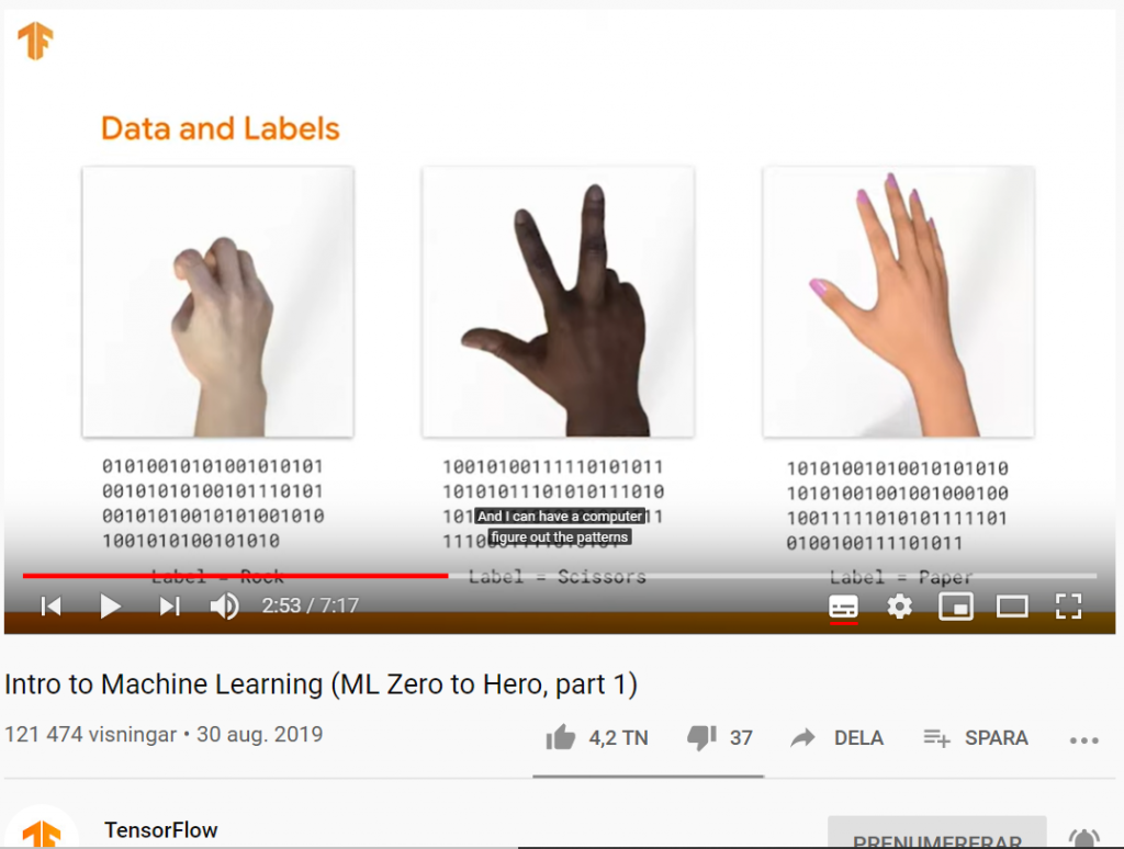
Maskininlärning (Machine Learning, ML) representerar ett nytt paradigm i programmering, där du istället för att programmera explicita regler på ett språk som Java eller C ++, bygger ett system som tränas och lärs upp på data från ett stort antal exempel, för att sedan kunna dra slutsatser av ny data baserat på de mönster som identifierats utifrån träningsdatat. Men hur ser ML egentligen ut? I del ett av Machine Learning Zero to Hero går AI-evangelisten Laurence Moroney (lmoroney @) genom ett grundläggande Hello World-exempel på hur man bygger en ML-modell och introducerar idéer som vi kommer att tillämpa i det senare avsnittet om datorseende (Computer Vision) längre ner på denna sida. Vill du ha en lite mer omfattande introduktion rekommenderar jag Introduction to TensorFlow 2.0: Easier for beginners, and more powerful for experts.
Prova själv den här koden i Hello World of Machine Learning: https://goo.gle/2Zp2ZF3
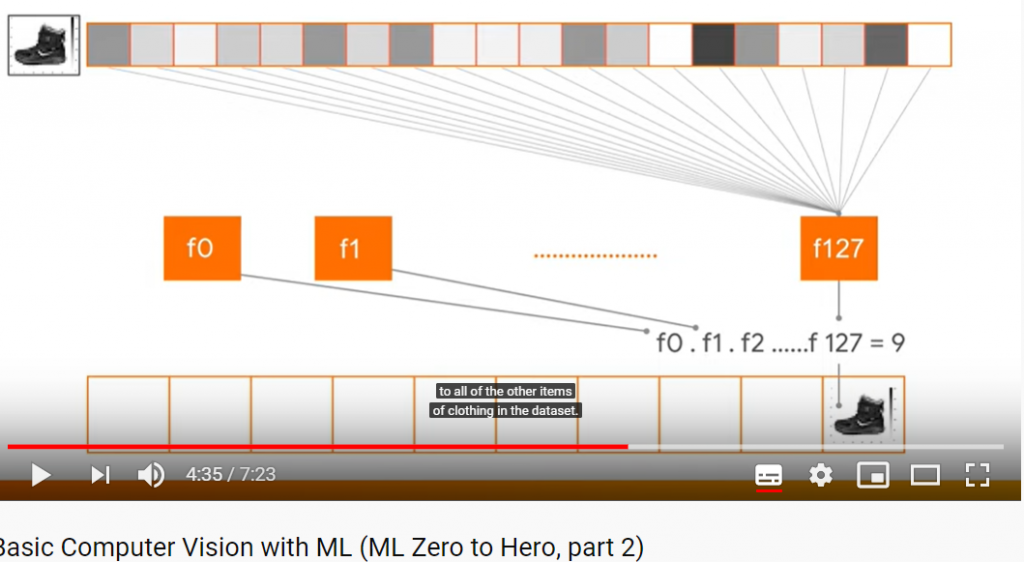
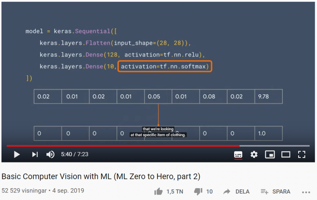
Basic Computer Vision with ML (ML Zero to Hero, part 2)
I del två av Machine Learning Zero to Hero går AI-evengalisten Laurence Moroney (lmoroney @) genom grundläggande datorseende (Computer Vision) med maskininlärning genom att lära en dator hur man ser och känner igen olika objekt (Object Recognition).
Fashion MNIST – ett dataset med bilder på kläder för benchmarking
Fashion-MNIST är ett forskningsprojekt av Kashif Rasul & Han Xiao i form av ett dataset av Zalandos artikelbilder. Det består av ett träningsset med 60 000 bildexempel och en testuppsättning med 10 000 exempel. Varje exempel är en 28 × 28 pixlar stor gråskalabild, associerad med en etikett från 10 klasser (klädkategorier). Fashion-MNIST är avsett att fungera som en direkt drop-in-ersättning av det ursprungliga MNIST-datasättet för benchmarking av maskininlärningsalgoritmer.
Fashion MNIST dataset
Varför är detta av intresse för det vetenskapliga samfundet?
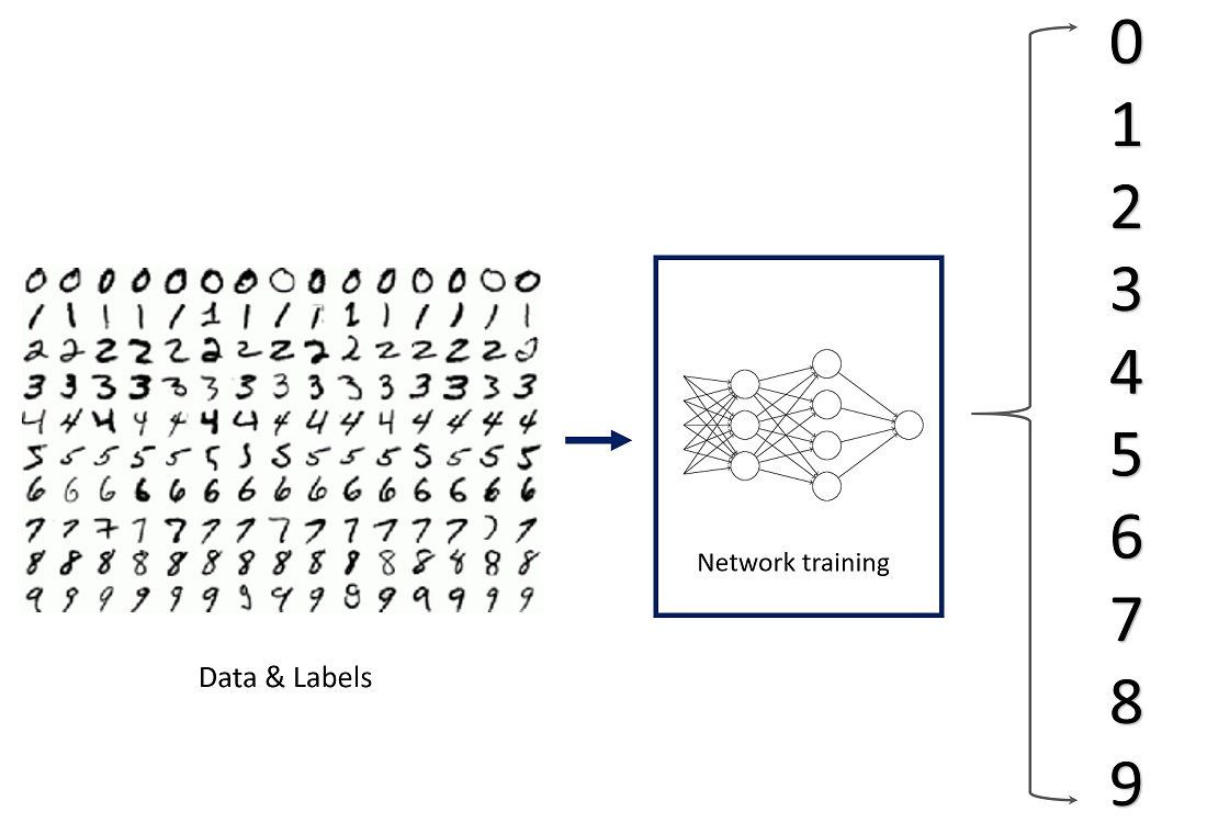
Det ursprungliga MNIST-datasättet innehåller många handskrivna siffror. Människor från AI / ML / Data Science community älskar detta dataset och använder det som ett riktmärke för att validera sina algoritmer. Faktum är att MNIST ofta är det första datasetet de provar på. ”Om det inte fungerar på MNIST, fungerar det inte alls”, sägs det. ”Tja, men om det fungerar på MNIST, kan det fortfarande misslyckas med andra.”
MNIST Dataset för nummerklassificering
Fashion-MNIST är avsett att tjäna som en direkt drop-in ersättning för det ursprungliga MNIST-datasetet för att benchmarka maskininlärningsalgoritmer, eftersom det delar samma bildstorlek och strukturen för tränings- och testdelningar.
Varför ska man ersätta MNIST med Fashion MNIST? Här är några goda skäl:
Se mer om att koda TensorFlow → https://bit.ly/Coding-TensorFlow Prenumerera på TensorFlow-kanalen → http://bit.ly/2ZtOqA3
Introducing convolutional neural networks (ML Zero to Hero, part 3)
I del tre av Machine Learning Zero to Hero diskuterar AI-evangelisten Laurence Moroney (lmoroney @) CNN-nätverk (Convolutional Neural Networks) och varför de är så kraftfulla i datorseende-scenarier. En ”convolution” är ett filter som passerar över en bild, bearbetar den och extraherar funktioner eller vissa kännetecken (features) i bilden. I den här videon ser du hur de fungerar genom att bearbeta en bild för att se om du kan hitta specifika kännetecken (features) i bilden.
Codelab: Introduktion till invändningar → http://bit.ly/2lGoC5f
Introducing convolutional neural networks (ML Zero to Hero, part 3)
Build an image classifier (ML Zero to Hero, part 4)
I del fyra av Machine Learning Zero to Hero diskuterar AI-evangelisten Laurence Moroney (lmoroney @) byggandet av en bildklassificerare för sten, sax och påse. I avsnitt ett visade vi ett scenario med sten, sax och påse, och diskuterade hur svårt det kan vara att skriva kod för att upptäcka och klassificera dessa. I de efterföljande avsnitten har vi lärt oss hur man bygger neurala nätverk för att upptäcka mönster av pixlarna i bilderna, att klassificera dem, och att upptäcka vissa kännetecken (features) med hjälp av bildklassificeringssystem med ett CNN-nätverk (Convolutional Neural Network). I det här avsnittet har vi lagt all information från de tre första delarna av serien i en.
Colab anteckningsbok: http://bit.ly/2lXXdw5
Rock, papper, saxdatasätt: http://bit.ly/2kbV92O
Build an image classifier (ML Zero to Hero, part 4)
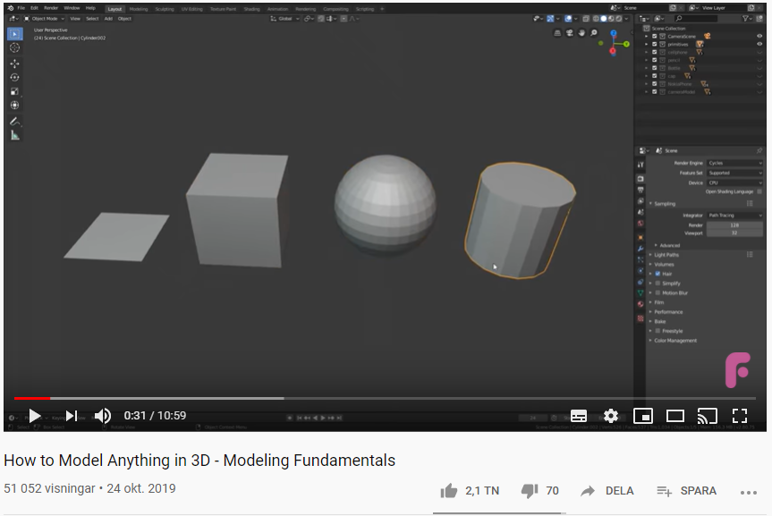
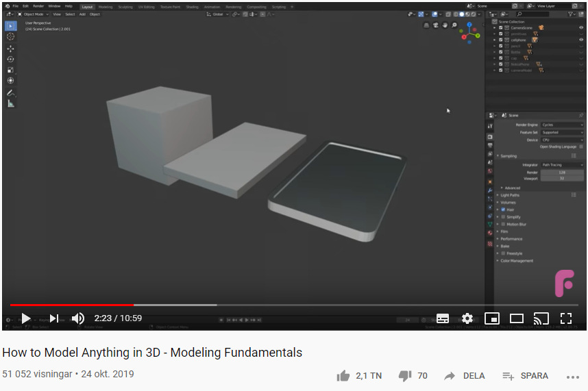
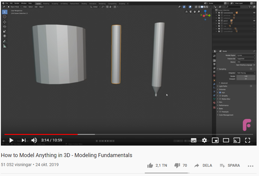
I denna tutorial får du lära dig en metod för att modellera nästan vad som helst i 3D. När du ska skissa, rita eller 3D-modellera ett objekt kan du kombinera och förändra de fyra grundformerna plan, kub, sfär och cylinder. I filmklippet används programvaran Blender, men samma principer gäller för alla 3D-programvaror.


